[OneAI Documentation](/s/user-guide-en) # AI Maker Case Study - Clara 4.0 Tutorial: Using Spleen CT Dataset to Train Model with 3D Segmentation Technology [TOC] ## 0. Introduction To facilitate the development of medical imaging-related services, AI Maker integrates **NVIDIA Clara** medical imaging AI with the HPC application framework to provide the software and hardware environment technologies required for the development and training process, allowing you to easily train and use medical imaging models. In this example, we will describe how to use a publicly available Computed Tomography (CT) dataset of the spleen to train 3D model with segmentation technology, and how to use the trained model for identification. The main steps are as follows: 1. [**Prepare MMAR and Dataset**]#1-Prepare-MMAR-and-Dataset) At this stage, we will describe how to obtain public MMARs and datasets and upload them to the designated location. 2. [**Train model with segmentation technology**](#2-train-model-with-segmentation-technology) At this stage, we will configure related training jobs for Clara training and fitting, and store the trained model. 3. [**Create Inference Service**](#3-create-inference-service) At this stage, we deploy the stored model to the inference service for inference. 4. [**AIAA Client**](#4-AIAA-client---3D-slicer) At this stage, we introduce how to use [**3D-Slicer**](#4-AIAA-client---3D-slicer) and [**Jupyter**](#5-AIAA-client---jupyter), two AIAA (AI Assisted Annotation) Clients to connect with the inference service for inference. After completing this example, you will have learned to: 1. Familiarize yourself with AI Maker functions and create jobs for each stage. 2. Use AI Maker's built-in templates to create related jobs. 3. Use the storage service and upload data. 4. How to connect with AIAA Server for inference. ## 1. Prepare MMAR and Dataset In this step, we describe how to prepare the Medical Model Archive (MMAR) and obtain the relative spleen dataset. ### 1.1 Upload MMAR Please follow the steps below to prepare MMAR and dataset. 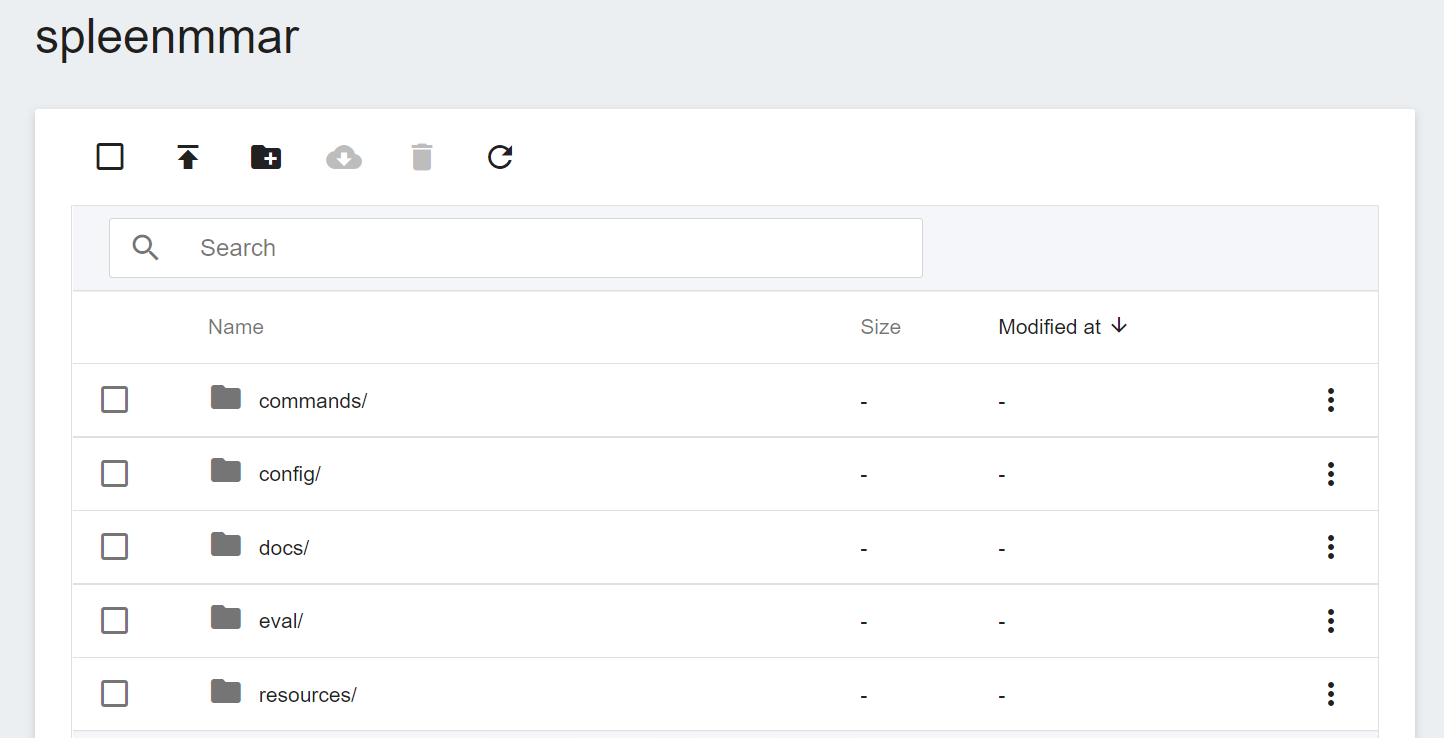First, we prepare the [Medical Model Archive (MMAR)](https://docs.nvidia.com/clara/tlt-mi_ea/clara-train-sdk-v4.0/nvmidl/mmar.html) file required in the Clara service. This file defines a standard structure, which is the data structure that Clara uses to arrange various tasks in the development life cycle. The standard MMAR data structure is as follows : ``` ./Project ├── commands ├── config ├── docs ├── eval ├── models └── resources ``` Here: 1. **commands**: This will contain the required scripts, usually training, multi-GPU training, validation, inference and TensorRT transformations...and more. 2. **config**: Contains configuration JSON files such as training, validation, AIAA deployment and environment... required for each training. 3. **docs**: As the name suggests, the place to put documents. 4. **eval**: eval preset result output directory. 5. **models**: The directory used to store the training model. The three most important directories are **commands**, **config** and **models**. In this example, instead of rewriting the MMAR file, we use a pretrained model [**clara_pt_spleen_ct_segmentation**](https://github.com/OneAILabs/ai-template-model/blob/master/clara_pt_spleen_ct_segmentation.zip) for 3D segmentation of spleen provided by NGC from CT images, and upload the spleen dataset to the storage service provided by the platform. 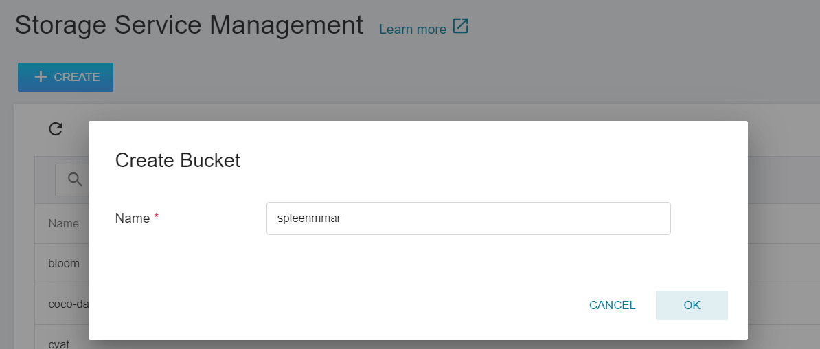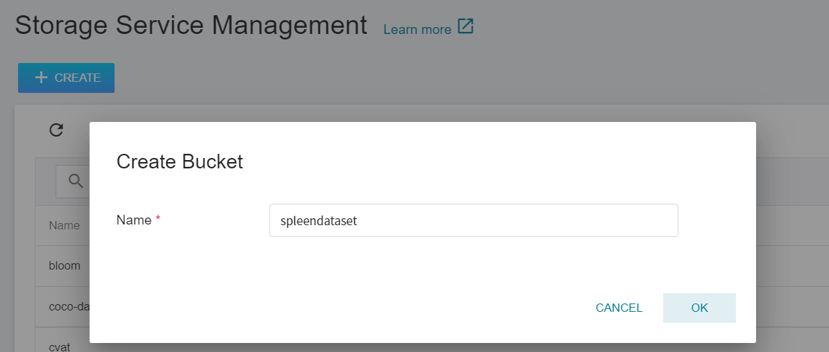1. **Create a Bucket** Select **Storage Service** from the OneAI service list to enter the storage service management page, and then click **+CREATE** to add a bucket named `spleenmmar` to store our MMAR files.  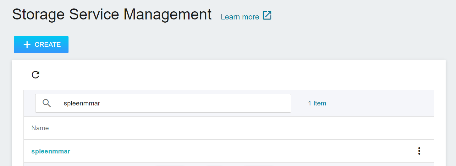2. **View Bucket** After the bucket is created, go back to the **Storage Service Management** page, and you will see that the bucket has been created.  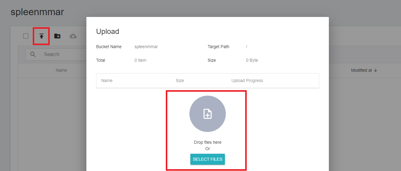3. **Upload MMAR** Click the created bucket, and then click **UPLOAD** to start uploading the dataset. (See [**Storage Service Documentation**](/s/storage-en)).   The core MMAR file is config_train.json under config. This JSON file contains all the parameters needed to define the neural network, the construction of the network model, the activation functions, the optimizer... and more. The settings required for Training and Validation are defined separately, and are described in detail in the official [**NVIDIA Documentation**](https://docs.nvidia.com/clara/clara-train-sdk/pt/appendix/configuration.html#training-configuration). ### 1.2 Upload Dataset After uploading the MMAR file, prepare the corresponding spleen dataset, and divide the dataset into Training Set and Validation Set according to the settings in **config_train.json**. We use the public dataset — [**Medical Segmentation Decathlon (Medical Segmentation Decathlon)**](http://medicaldecathlon.com/) for training, from which we download **`Task09_Spleen.tar`**. This is a competition dataset for semantic segmentation of medical images, and this Task09 is a dataset for the spleen. :::info :bulb: **Tips:** Please read the relevant instructions on the [**NGC Website**](https://catalog.ngc.nvidia.com/orgs/nvidia/teams/med/models/clara_pt_spleen_ct_segmentation) in detail, and perform the necessary data preprocessing. ::: <center> <img src="/uploads/o33Cg55.png" alt="Introduction to the Spleen Dataset"></center> <center>Introduction to the Spleen Dataset</center> <center><a href="http://medicaldecathlon.com/">(Image Credit: Medical Segmentation Decathlon)</a></center> <br><br> Once the dataset is ready, divide the dataset into Training Set and Validation Set and upload them to the storage service. 1. **Training Set and Validation Set** There will be a **dataset.json** in this dataset, and this json file defines how to slice the dataset. However, only Training Set and Test Set are defined in this file, so we need to slice out Validation Set from Training Set. We add a **`validation`** key to the json; its value is an array whose contents are the data we moved from the Training Set. ```json "validation":[ {"image":"./imagesTr/spleen_19.nii.gz","label":"./labelsTr/spleen_19.nii.gz"}, {"image":"./imagesTr/spleen_31.nii.gz","label":"./labelsTr/spleen_31.nii.gz"}, {"image":"./imagesTr/spleen_52.nii.gz","label":"./labelsTr/spleen_52.nii.gz"}, {"image":"./imagesTr/spleen_40.nii.gz","label":"./labelsTr/spleen_40.nii.gz"}, {"image":"./imagesTr/spleen_3.nii.gz","label":"./labelsTr/spleen_3.nii.gz"}, {"image":"./imagesTr/spleen_17.nii.gz","label":"./labelsTr/spleen_17.nii.gz"}, {"image":"./imagesTr/spleen_21.nii.gz","label":"./labelsTr/spleen_21.nii.gz"}, {"image":"./imagesTr/spleen_33.nii.gz","label":"./labelsTr/spleen_33.nii.gz"}, {"image":"./imagesTr/spleen_9.nii.gz","label":"./labelsTr/spleen_9.nii.gz"}, {"image":"./imagesTr/spleen_29.nii.gz","label":"./labelsTr/spleen_29.nii.gz"}], ``` <br> The complete content after revision is as follows: :::spoiler **dataset.json** ```json { "name": "Spleen", "description": "Spleen Segmentation", "reference": "Memorial Sloan Kettering Cancer Center", "licence":"CC-BY-SA 4.0", "release":"1.0 06/08/2018", "tensorImageSize": "3D", "modality": { "0": "CT" }, "labels": { "0": "background", "1": "spleen" }, "numTraining": 41, "numTest": 20, "training":[ {"image":"./imagesTr/spleen_46.nii.gz","label":"./labelsTr/spleen_46.nii.gz"}, {"image":"./imagesTr/spleen_25.nii.gz","label":"./labelsTr/spleen_25.nii.gz"}, {"image":"./imagesTr/spleen_13.nii.gz","label":"./labelsTr/spleen_13.nii.gz"}, {"image":"./imagesTr/spleen_62.nii.gz","label":"./labelsTr/spleen_62.nii.gz"}, {"image":"./imagesTr/spleen_27.nii.gz","label":"./labelsTr/spleen_27.nii.gz"}, {"image":"./imagesTr/spleen_44.nii.gz","label":"./labelsTr/spleen_44.nii.gz"}, {"image":"./imagesTr/spleen_56.nii.gz","label":"./labelsTr/spleen_56.nii.gz"}, {"image":"./imagesTr/spleen_60.nii.gz","label":"./labelsTr/spleen_60.nii.gz"}, {"image":"./imagesTr/spleen_2.nii.gz","label":"./labelsTr/spleen_2.nii.gz"}, {"image":"./imagesTr/spleen_53.nii.gz","label":"./labelsTr/spleen_53.nii.gz"}, {"image":"./imagesTr/spleen_41.nii.gz","label":"./labelsTr/spleen_41.nii.gz"}, {"image":"./imagesTr/spleen_22.nii.gz","label":"./labelsTr/spleen_22.nii.gz"}, {"image":"./imagesTr/spleen_14.nii.gz","label":"./labelsTr/spleen_14.nii.gz"}, {"image":"./imagesTr/spleen_18.nii.gz","label":"./labelsTr/spleen_18.nii.gz"}, {"image":"./imagesTr/spleen_20.nii.gz","label":"./labelsTr/spleen_20.nii.gz"}, {"image":"./imagesTr/spleen_32.nii.gz","label":"./labelsTr/spleen_32.nii.gz"}, {"image":"./imagesTr/spleen_16.nii.gz","label":"./labelsTr/spleen_16.nii.gz"}, {"image":"./imagesTr/spleen_12.nii.gz","label":"./labelsTr/spleen_12.nii.gz"}, {"image":"./imagesTr/spleen_63.nii.gz","label":"./labelsTr/spleen_63.nii.gz"}, {"image":"./imagesTr/spleen_28.nii.gz","label":"./labelsTr/spleen_28.nii.gz"}, {"image":"./imagesTr/spleen_24.nii.gz","label":"./labelsTr/spleen_24.nii.gz"}, {"image":"./imagesTr/spleen_59.nii.gz","label":"./labelsTr/spleen_59.nii.gz"}, {"image":"./imagesTr/spleen_47.nii.gz","label":"./labelsTr/spleen_47.nii.gz"}, {"image":"./imagesTr/spleen_8.nii.gz","label":"./labelsTr/spleen_8.nii.gz"}, {"image":"./imagesTr/spleen_6.nii.gz","label":"./labelsTr/spleen_6.nii.gz"}, {"image":"./imagesTr/spleen_61.nii.gz","label":"./labelsTr/spleen_61.nii.gz"}, {"image":"./imagesTr/spleen_10.nii.gz","label":"./labelsTr/spleen_10.nii.gz"}, {"image":"./imagesTr/spleen_38.nii.gz","label":"./labelsTr/spleen_38.nii.gz"}, {"image":"./imagesTr/spleen_45.nii.gz","label":"./labelsTr/spleen_45.nii.gz"}, {"image":"./imagesTr/spleen_26.nii.gz","label":"./labelsTr/spleen_26.nii.gz"}, {"image":"./imagesTr/spleen_49.nii.gz","label":"./labelsTr/spleen_49.nii.gz"}], "validation":[ {"image":"./imagesTr/spleen_19.nii.gz","label":"./labelsTr/spleen_19.nii.gz"}, {"image":"./imagesTr/spleen_31.nii.gz","label":"./labelsTr/spleen_31.nii.gz"}, {"image":"./imagesTr/spleen_52.nii.gz","label":"./labelsTr/spleen_52.nii.gz"}, {"image":"./imagesTr/spleen_40.nii.gz","label":"./labelsTr/spleen_40.nii.gz"}, {"image":"./imagesTr/spleen_3.nii.gz","label":"./labelsTr/spleen_3.nii.gz"}, {"image":"./imagesTr/spleen_17.nii.gz","label":"./labelsTr/spleen_17.nii.gz"}, {"image":"./imagesTr/spleen_21.nii.gz","label":"./labelsTr/spleen_21.nii.gz"}, {"image":"./imagesTr/spleen_33.nii.gz","label":"./labelsTr/spleen_33.nii.gz"}, {"image":"./imagesTr/spleen_9.nii.gz","label":"./labelsTr/spleen_9.nii.gz"}, {"image":"./imagesTr/spleen_29.nii.gz","label":"./labelsTr/spleen_29.nii.gz"}], "test":["./imagesTs/spleen_15.nii.gz", "./imagesTs/spleen_23.nii.gz", "./imagesTs/spleen_1.nii.gz", "./imagesTs/spleen_42.nii.gz", "./imagesTs/spleen_50.nii.gz", "./imagesTs/spleen_54.nii.gz", "./imagesTs/spleen_37.nii.gz", "./imagesTs/spleen_58.nii.gz", "./imagesTs/spleen_39.nii.gz", "./imagesTs/spleen_48.nii.gz", "./imagesTs/spleen_35.nii.gz", "./imagesTs/spleen_11.nii.gz", "./imagesTs/spleen_7.nii.gz", "./imagesTs/spleen_30.nii.gz", "./imagesTs/spleen_43.nii.gz", "./imagesTs/spleen_51.nii.gz", "./imagesTs/spleen_36.nii.gz", "./imagesTs/spleen_55.nii.gz", "./imagesTs/spleen_57.nii.gz", "./imagesTs/spleen_34.nii.gz"] } ``` ::: After revising the revised **dataset.json**, re-compress the folder into **Task09_Spleen.tar**, so that we can upload it easily. 2. **Create a Bucket** Next, similar to the steps for creating the **`spleenmmar`** bucket, we create a bucket called **`spleendataset`** in which we will place the spleen dataset.  3. **Upload Dataset** Next, decompress **Task09_Spleen.tar** on the local side and upload it to the bucket.  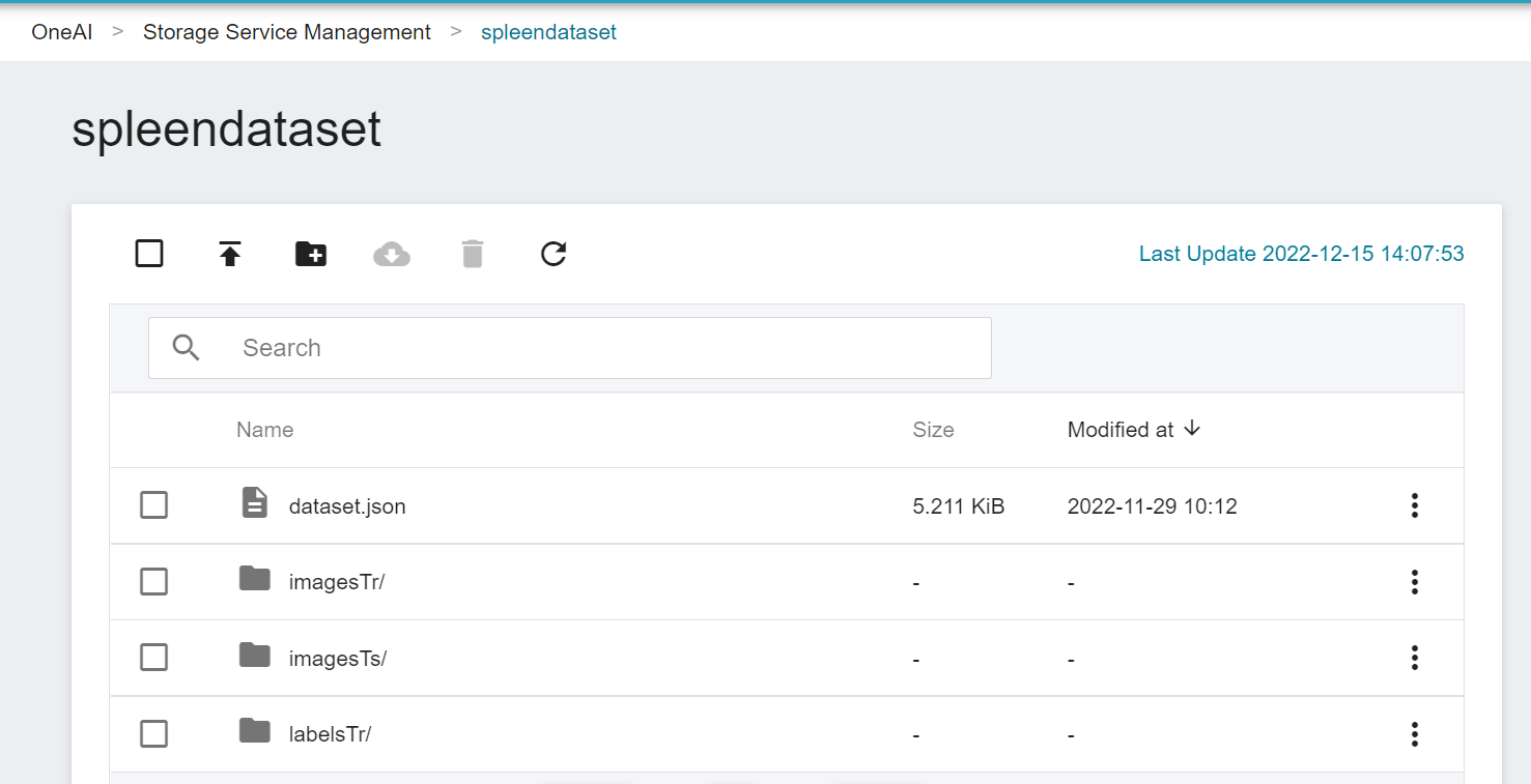Now, we have finished uploading the dataset. ## 2. Train the Segmentation Technology Model After completing the upload of [**MMAR**](#12-upload-MMAR) and [**Dataset**](#13-upload-dataset), we can use this dataset for transfer learning training. ### 2.1 Create Training Jobs Select **AI Maker** from the OneAI service list, and then click **Training Jobs**. After entering the training job management page, click **+CREATE** to add a training job.  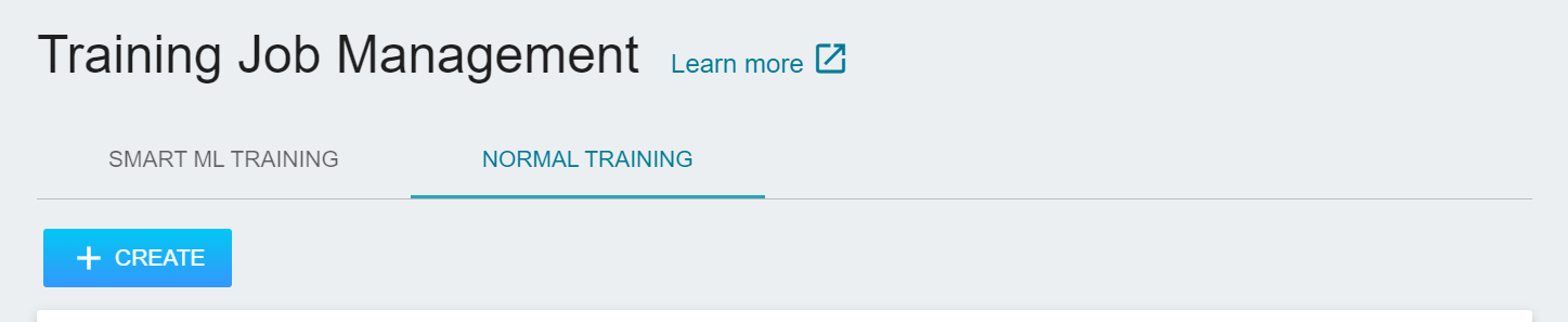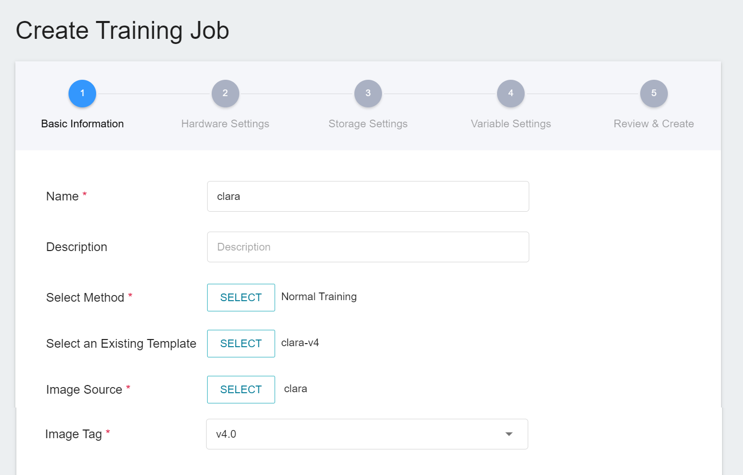#### 2.1.1 Normal Training Jobs There are five steps in creating a training job: 1. **Basic Information** The first step is to set the basic information. Please enter the **Name**, **Description**, and **Select Method** in sequence. In this section, we first select **`Normal Training Jobs`**. In addition, the rest of the information can be quickly brought into each setting by selecting a template that has already been created through the **Select Template** function. AI Maker provides a set of **`clara-v4`** templates for the training and use of Clara 4.0, which defines the variables and settings required for each stage, so that developers can quickly develop their own network. At this stage, we use the built-in **`clara-v4`** template to bring in various settings.  2. **Hardware Settings** Select the appropriate hardware resource from the list with reference to the current available quota and training program requirements. :::info :bulb: **Tips:** It is recommended to choose hardware with **Shared Memory** to avoid training failure due to insufficient resources. 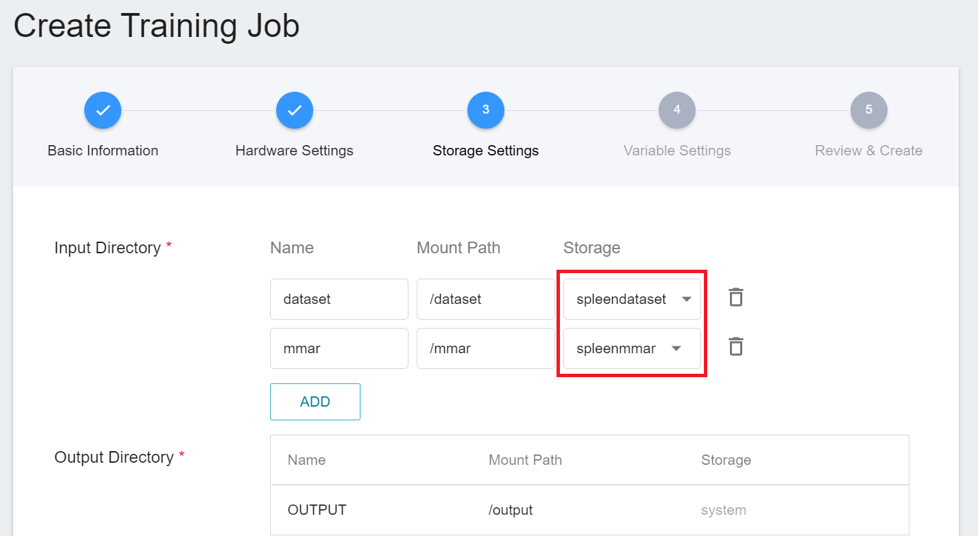::: 3. **Storage Settings** There are two buckets to be mounted at this stage: 1. **dataset**: the bucket **`spleendataset`** where we store data. 2. **mmar**: **`spleenmmar`**.  4. **Variable Settings** The variable settings step is to set environment variables and commands. The description of each field is as follows: | Field name | Description| | ------- | ----- | | Environment Variables | Enter the name and value of the environment variables. The environment variables here include settings related to the training execution as well as the parameters required for the training network.| | Target Parameter | After training, a value will be returned as the final result. Here, the name and target direction are set for the returned value. For example, if the returned value is the accuracy rate, you can name it accuracy and set its target direction to the maximum value; if the returned value is the error rate, you can name it error and set its direction to the minimum value.| | Command | Enter the command or program name to be executed. 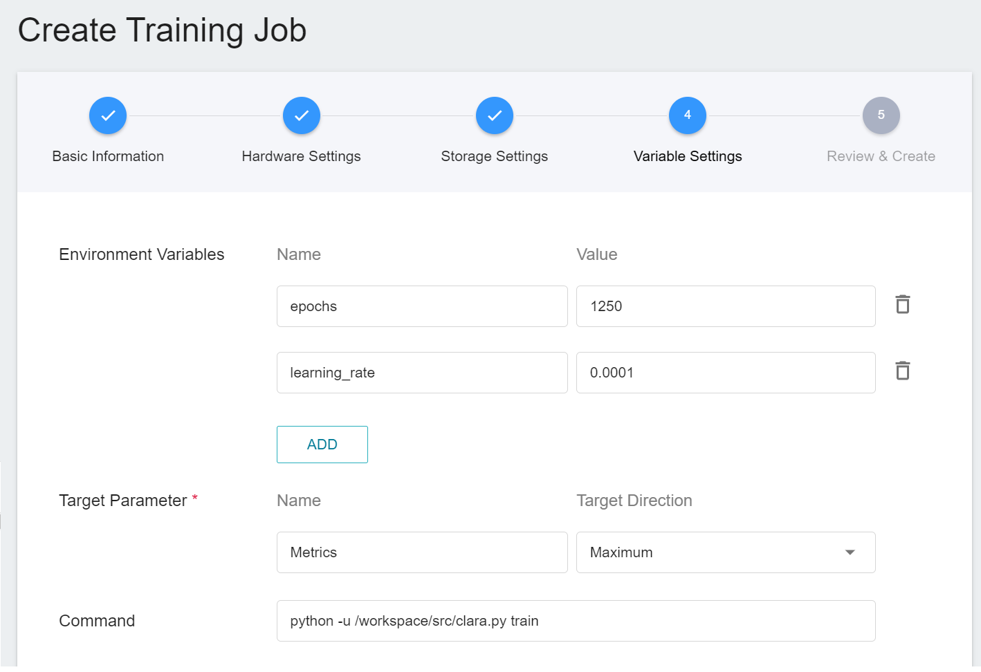For example: `python train.py`.| However, because we have applied the **`clara-v4`** template when filling in the basic information, these commands and parameters will be automatically imported:  The setting values of environment variables can be adjusted according to your development needs. Here are the descriptions of each environment variable: | Variable | Default | Description | | ------------- | ---------- | ---- | | epochs | Defined by config_train.json | One epoch = one forward pass and one backward pass for all training samples.| | learning_rate | Defined by config_train.json | The **Learning Rate** parameter can be set larger at the beginning of model learning to speed up the training. In the later stage of learning, it needs to be set smaller to avoid divergence. | In addition, the neural network parameters, optimizers and other settings in MMAR can also be adjusted through environment variables, for example: 1. To modify the network loss function, we can use **`train.loss.name`** as the environment variable in MMAR's **config_train.json**. 2. To modify the network optimizer, the environment variable **`train.optimizer.name`** can be specified. Please refer to [**NVIDIA's MMAR Documentation**](https://docs.nvidia.com/clara/tlt-mi_ea/clara-train-sdk-v4.0/nvmidl/appendix/configuration.html) for the selection of values for each of the environment variables. 5. **Review & Create** Finally, confirm the entered information and click CREATE. #### 2.1.2 Smart ML Training Jobs In the [**previous section**](#211-Normal-Training-Jobs), we introduced the creation of **Normal Training Jobs**, and here we introduce the creation of **Smart ML Training Jobs**. You can choose just one training method or compare the differences between the two. Both processes are roughly the same, but there are additional parameters to be set, and only the additional variables are described here. 1. 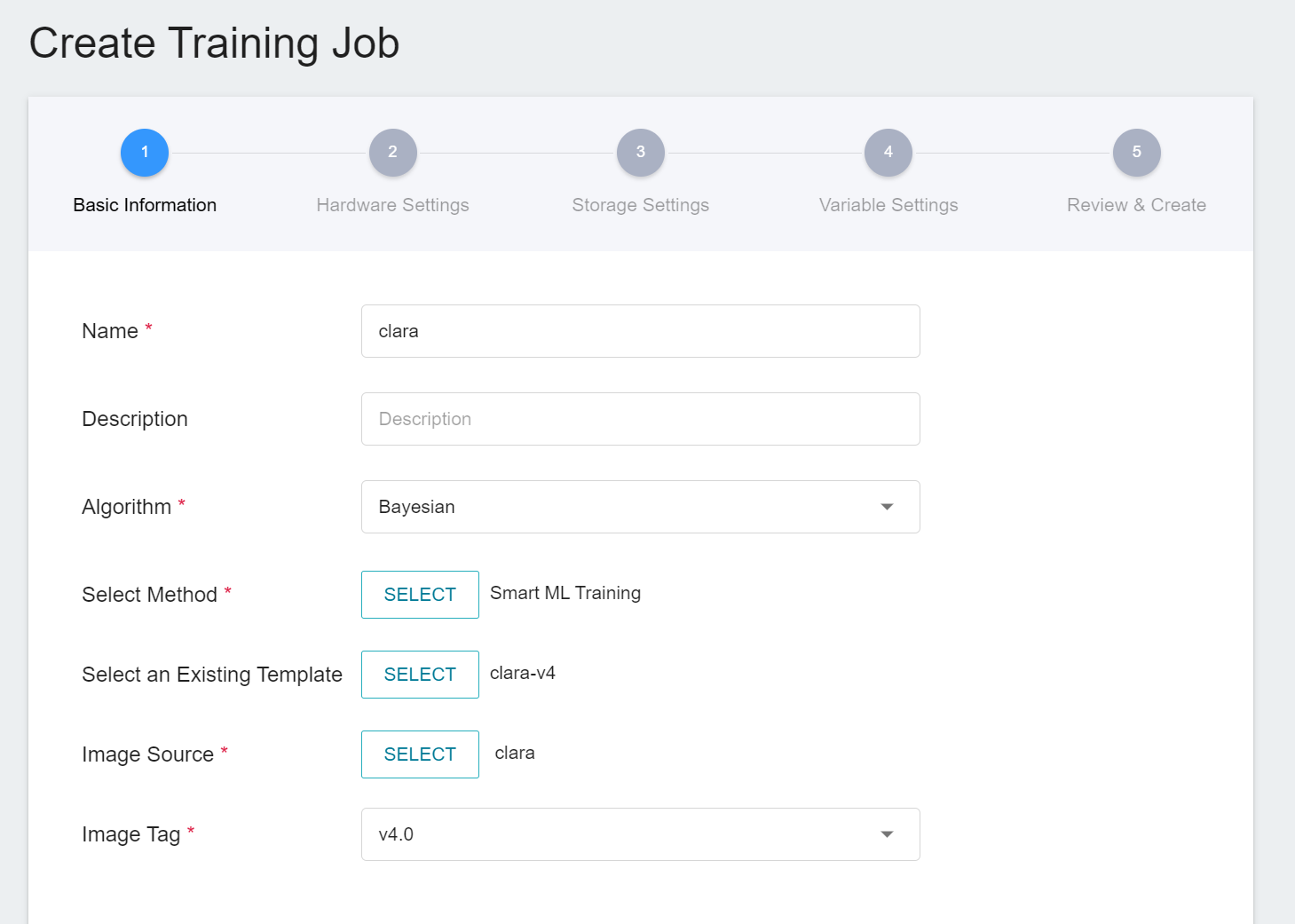**Basic Information**  When Smart ML training job is the setting method, you will be further required to select the **Algorithm** to be used for the Smart ML training job, and the algorithms that can be selected are as follows. - **Bayesian**: Efficiently perform multiple training jobs to find better parameter combinations, depending on environmental variables, the range of hyperparameter settings, and the number of training sessions. - **TPE**: Tree-structured Parzen Estimator, similar to the Bayesian algorithm, can optimize the training jobs of high-dimensional hyperparameters. - **Grid**: Experienced machine learning users can specify multiple values of hyperparameters, and the system will perform multiple training jobs based on the combination of the hyperparameter lists and obtain the calculated results. - **Random**: Randomly select hyperparameters for the training job within the specified range. 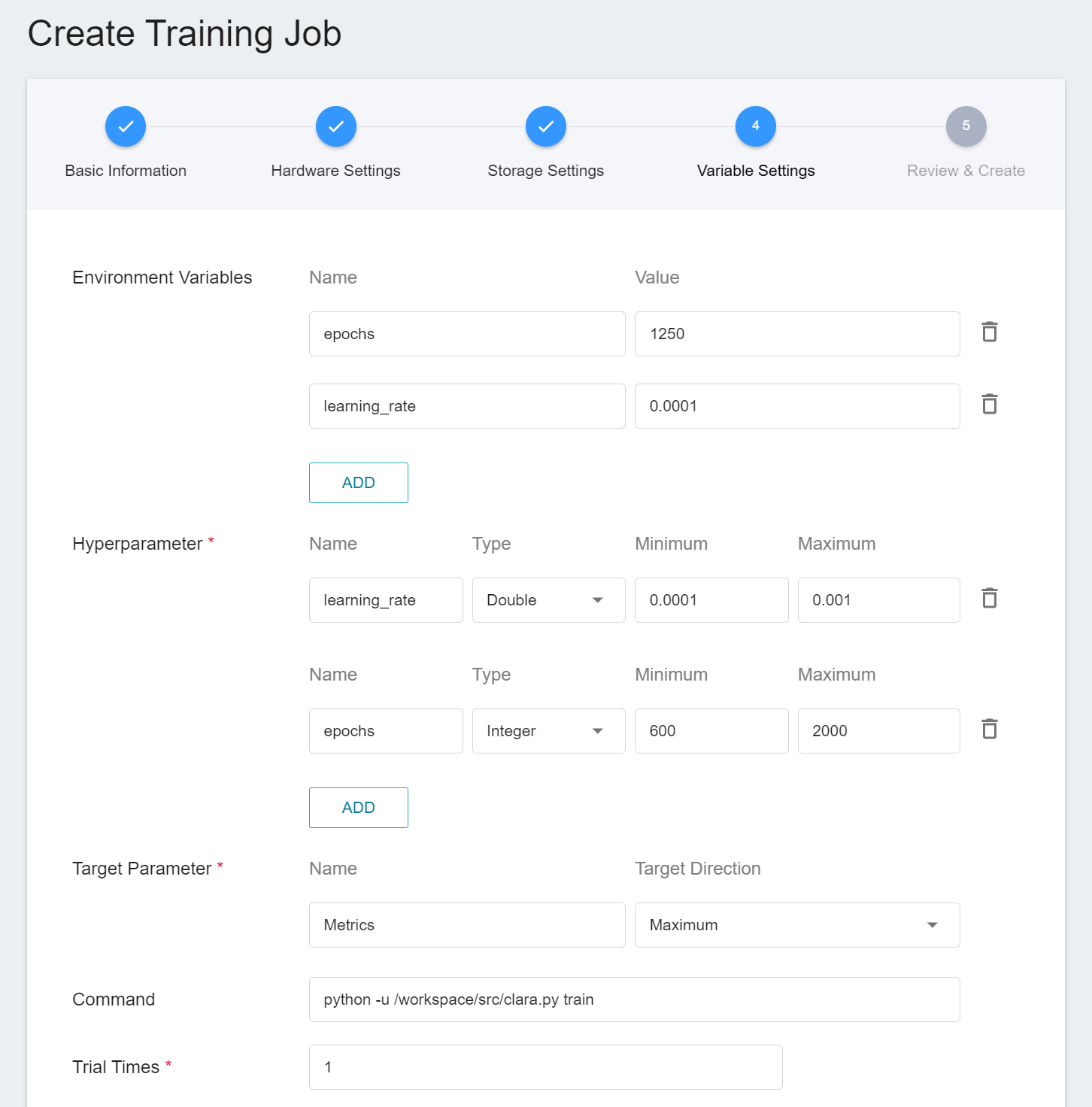2. **Variable Settings** In the variable settings page, there will be additional settings for **Hyperparameter** and **Trial Times**: - **Hyperparameter** This tells the job what parameters to try. Each parameter must have a name, type, and value (or range of values) when it is set. After selecting the type (integer, float, and array), enter the corresponding value format when prompted. - **Trial Times** Set the number of training sessions, and the training job is executed multiple times to find a better parameter combination.  Of course, some of the training parameters in **Hyperparameter** can be moved to **Environmental Variables** and vice versa. If you want to fix a parameter, you can remove it from the hyperparameter setting and add it to the environment variable with a fixed value; conversely, if you want to add the parameter to the trial, remove it from the environment variable and add it to the hyperparameter settings below. ### 2.2 Start a Training Job After completing the setting of the training job, go back to the training job management page, and you can see the job you just created.  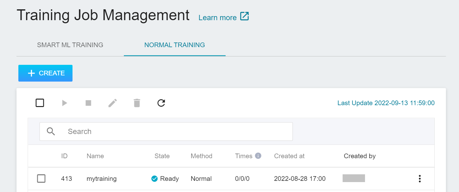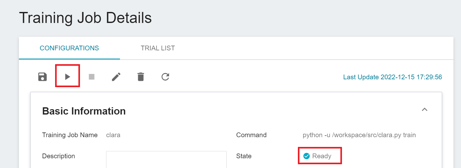Click the job to view the detailed settings of the training job. In the command bar, there are 6 icons. If the job state is displayed as **`Ready`** at this time, you can click **START** to execute the training job.  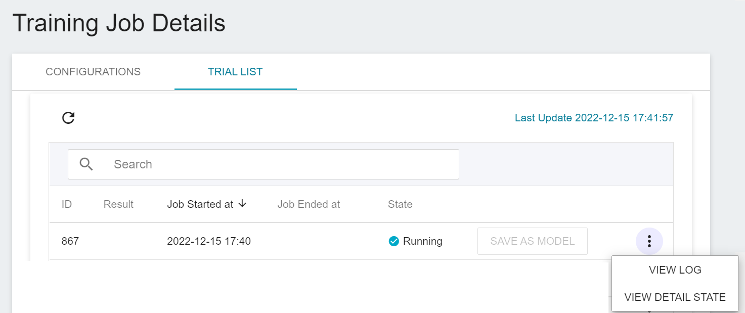Once started, click the **Trial List** tab above to view the execution status and schedule of the job in the list. During training, you can click **VIEW LOG** or **VIEW DETAIL STATE** in the list on the right of the job to know the details of the current job execution.  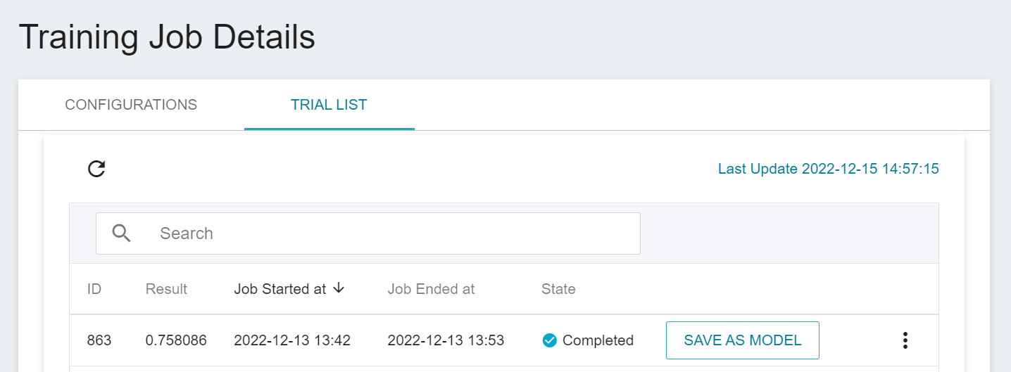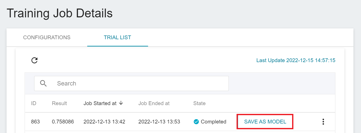### 2.3 View Training Results And Save Model After the training job is completed, the job state in the Trial List page will change to **`Completed`** and the result will be displayed.  After training, the models with expected scores are stored in the **Model Repository**; if the scores are not satisfactory, the values or range of values for the environment variables and hyperparameters are readjusted until a suitable model appears. Below is a description of how to save the expected model to the model repository: 1. **Click Save as Model** Click the **SAVE AS MODEL** button to the right of the training result you want to save.  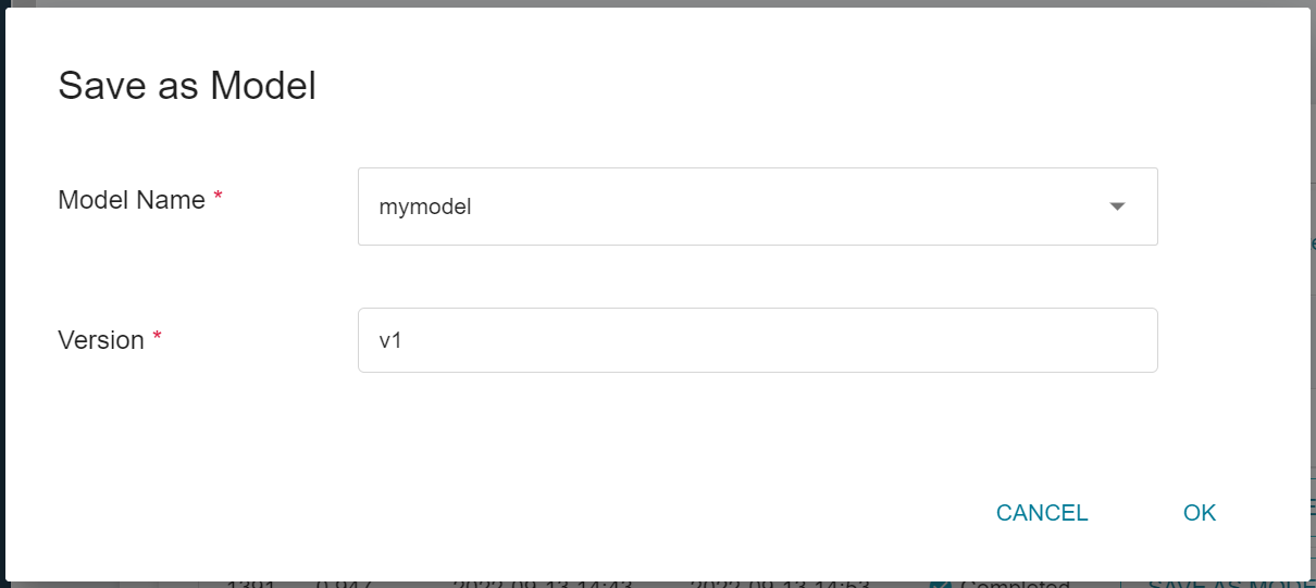2. **Enter the Model Name and Version Number** A dialog box will appear, follow the instructions to enter the model name and version, and click OK when finished.  :::info :alarm_clock: **Small Reminder:** This trained model is slightly larger, it will take some time to save, please be patient. 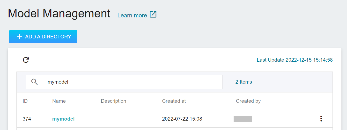::: 3. **View the Model** Select **AI Maker** from the OneAI service list, and then click **MODEL**. After entering the model management page, you can find the model in the list.  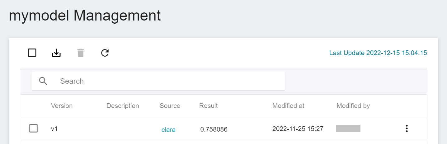Click the model to enter the version list of the model, where you can see all the version numbers of the stored model, the corresponding training jobs and results... and other information.  ## 3. Create Inference Service After training the segmentation technology model, we can deploy the **Inference Feature** to set up the AIAA Server (AIAA-AI assisted annotation server). <center> <img src="/uploads/WIPLz1J.png" alt="AIAA"></center> <center>AIAA (Image Credit: NVIDIA）</center> <br> ### 3.1 Create Inference Select **AI Maker** from the OneAI service list, then click **INFERENCE** to enter the inference management page, and click **+CREATE** to create an inference job. 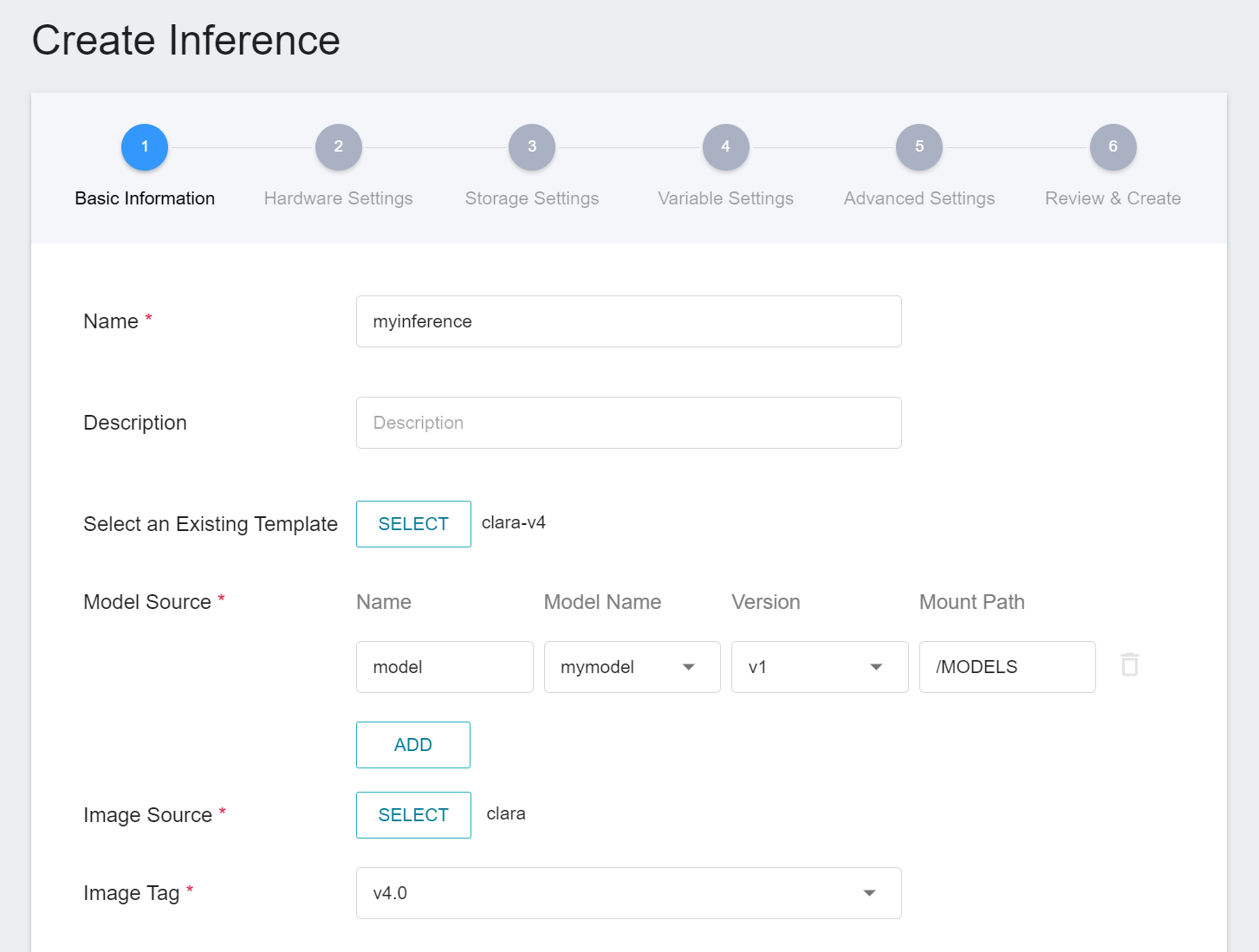The steps for creating the inference service are described below: 1. **Basic Information** Similar to the setting of basic information for training jobs, we also use the **`clara-v4`** inference template to facilitate quick setup for developers. However, the model name and version number to be loaded still need to be set manually by the user: - **Name** The file name of the loaded model relative to the program's ongoing read. This value will be set by the **`clara-v4`** inference template. - **Model Name** The name of the model to be loaded, that is, the model we saved in [**2.3 View training results and save model**](#23-View-Training-Results-And-Save-Model). - **Version** The version number of the model to be loaded is also the version number set in [**2.3 View training results and save model**](#23-View-Training-Results-And-Save-Model). - **Mount Path** The location of the model after loading relative to the program's ongoing read, this value will be set by the **`clara-v4`** inference template.  2. **Hardware Settings** Select the appropriate hardware resource from the list with reference to the current available quota and training program requirements. 3. **Storage Settings** No configuration is required for this step. 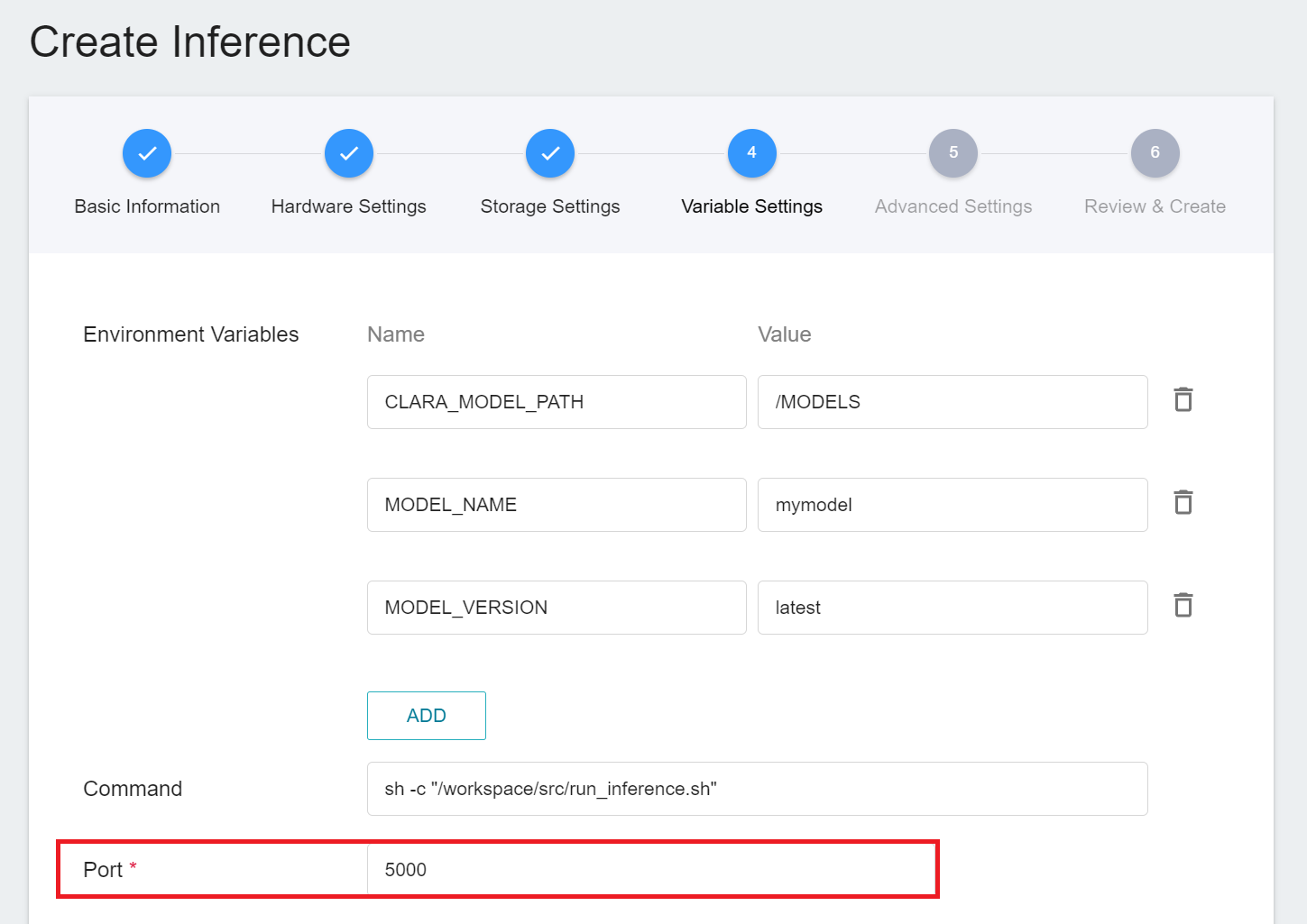4. **Variable Settings** In the variable settings step, the relevant variables will be automatically imported by the **`clara-v4`** template. Please set the **`Port`** to 5000.  5. **Advanced Settings** No configuration is required for this step. 6. **Review & Create** Finally, confirm the entered information and click CREATE. ### 3.2 Querying Inference Information After creating an inference job, go back to the inference management page and click the job you just created to view the detailed settings of the service. When the service state shows as **`Ready`**, you can start inference with the AIAA Client. 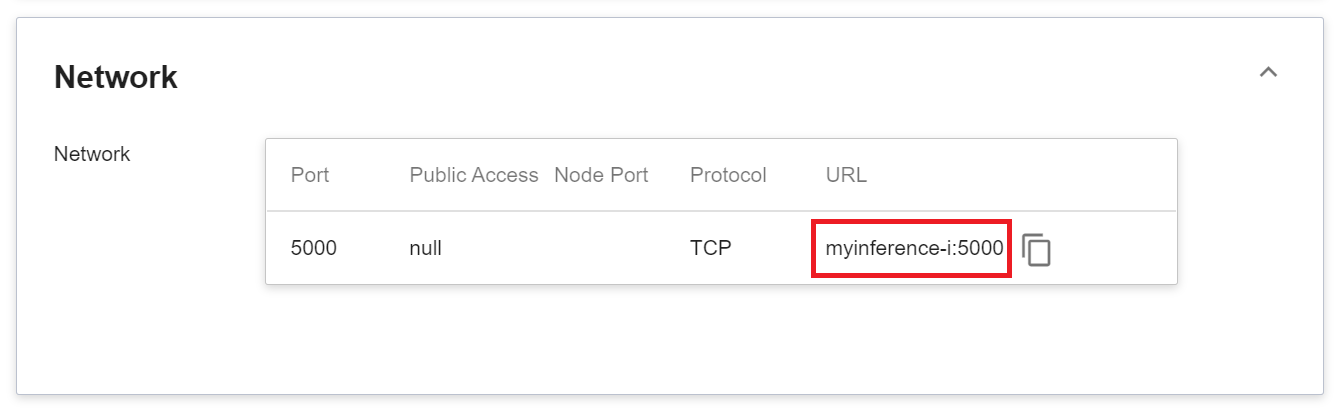However, you should be aware of some information in these details, as they will be used later when using the AIAA Client: 1. **Network** Since the current inference service does not have a public service port for security reasons, we can communicate with the inference service we created through the **Container Service**. The way to communicate is through the **URL** provided by the inference service, which will be explained in the next section. :::info :bulb: **Tips:** The URLs in the document are for reference only, and the URLs you got may be different. 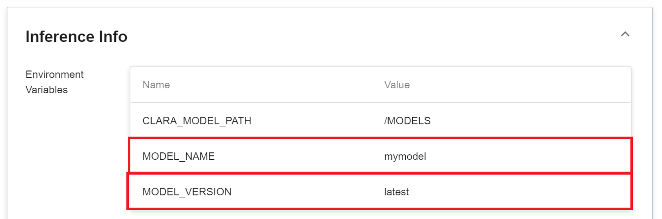:::  2. **Model** Another thing to note is that the **MODEL_NAME** and **MODLE_VERSION** in the environment variables are the name of the model and version number we imported in the program, or inside the service.  <br><br> ## 4. AIAA Client - 3D Slicer When you have finished starting the inference service, you have also finished starting the AIAA Server, so that you can work on the local AIAA Client. Here we use [**3D Slicer**](https://www.slicer.org/) as an example to demonstrate how to connect with the inference service. If you have any questions about the download and installation of 3D Slicer, please refer to the official [**3D Slicer Website**](https://download.slicer.org/). ### 4.1 **Create Container Service** Since the inference service does not open public service port for security reasons, we need to communicate with the inference service we created through the container service. Click **Container Service** from the OneAI service list to enter the container service management page, and click **+CREATE**. 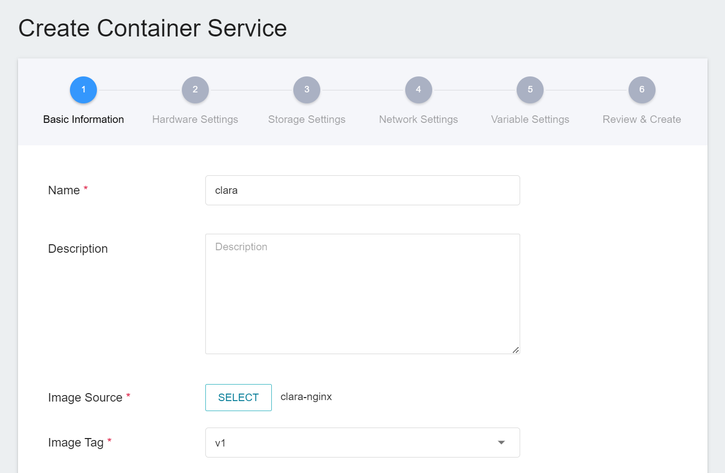1. Basic information When creating a container service, you can directly select the **`clara-nginx`** image.  2. **Hardware Settings** Select the hardware settings. Take into consideration of resource usage when selecting the resources, it is not necessary to configure GPU. 3. **Storage Settings** No configuration is required for this step. 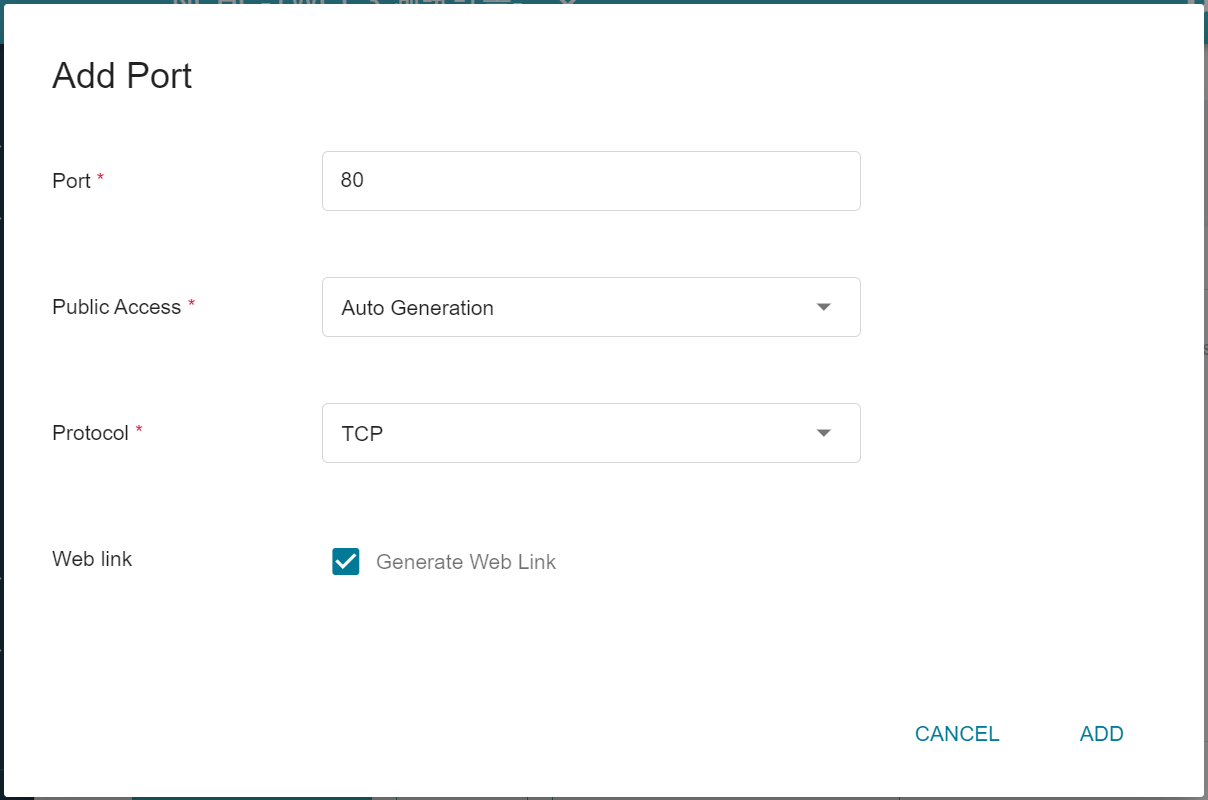4. **Network Settings** Please set **Allow Port** to **80**, it will automatically generate a public service port, and check **Generate Web Link**.  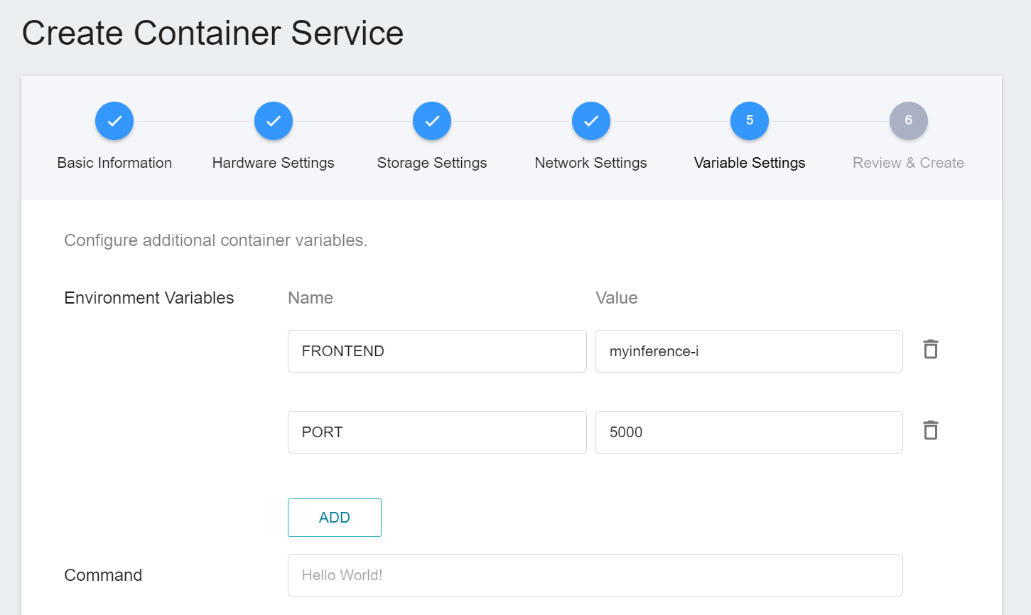5. **Variable Settings** Two new environment variables **`FRONTEND`** and **`PORT`** are added and set according to the Web Link obtained by the inference service. In this example **`FRONTEND`** is **`myinference-i`** and **`PORT`** is `5000`.  6. **Review & Create** Finally, confirm the entered information and click CREATE. 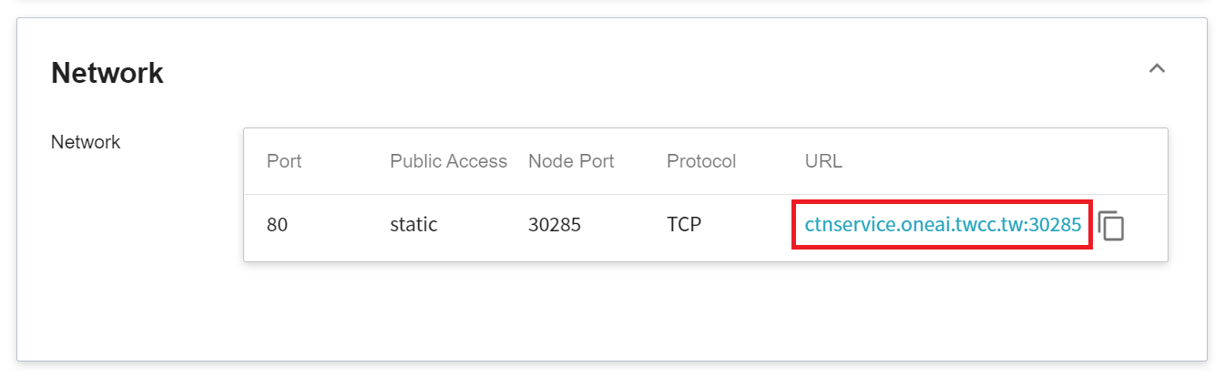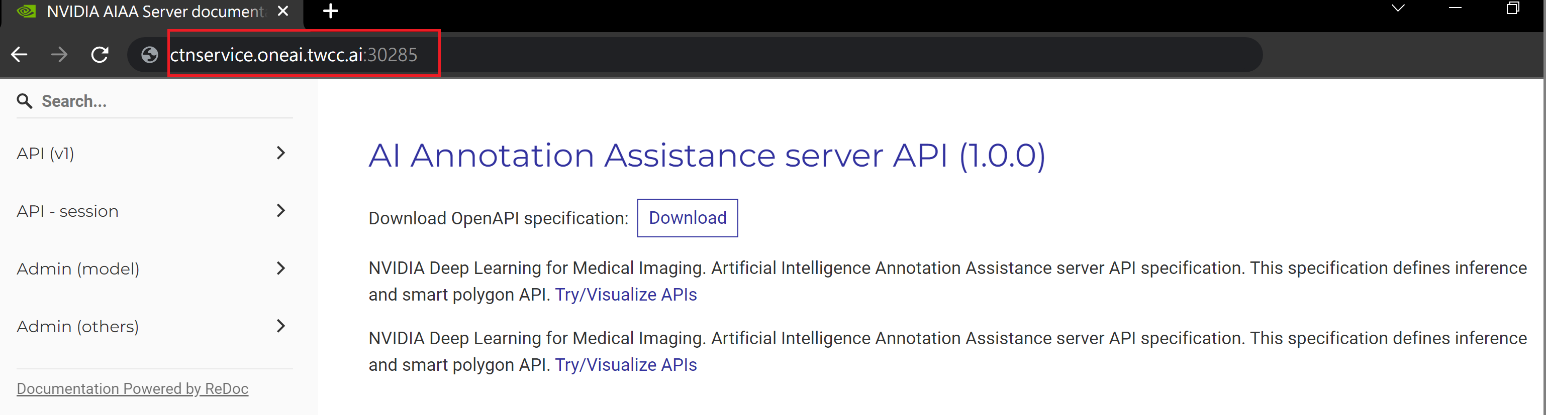7. **View Public Access** After creating the container service, go back to the container service management list page and click on the service to get detailed information. Please pay attention to the URL in the red box in the figure below. This is the public service URL of **NVIDIA AIAA Server**. Click this URL link to confirm whether the NVIDIA AIAA Server service is started normally in the browser tab; click the **Copy** icon on the right to copy this URL link , and next will introduce how to **Use 3D Slicer**.   ### 4.2 **Use 3D Slicer** :::info :bulb: **Tips:** The following 3D Slicer setup screen is based on version 4.11. If you are using other versions, please refer to the official [**3D Slicer Website**](https://www.slicer.org/) for instructions. 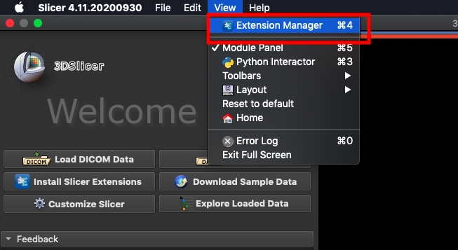::: 1. **Install NVIDIA Plug-in** The NVIDIA Plug-in needs to be installed first before proceeding to the other steps. Open 3D Slicer and click **`View` > `Extension Manager`**.  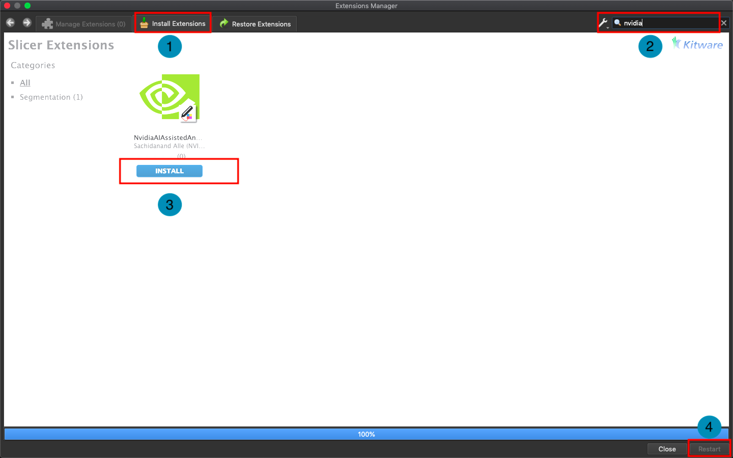Click **`Install Extensions`** and search for `nvidia`. At this point, the AI-Assisted Annotation Extension of NVIDIA Clara will appear, please click to install and restart 3D Slicer.  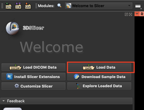2. 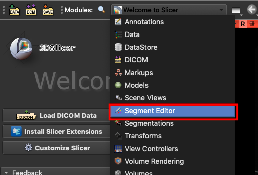**Load Data for Segmentation** Next, click **`Load Data`** to load the spleen data for segmentation.  and bring up the **`Segment Editor`**.  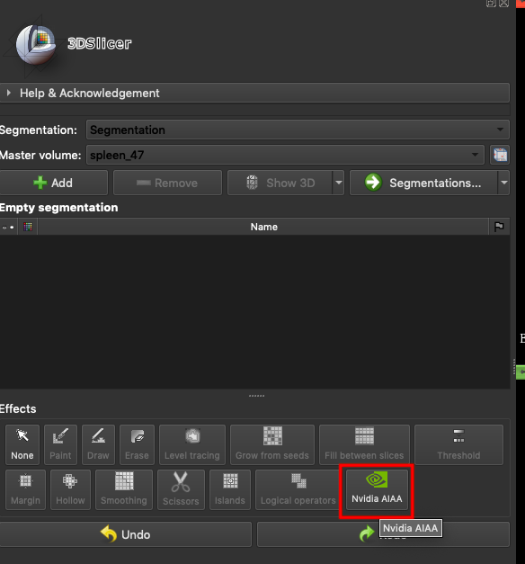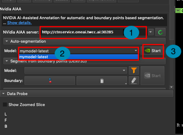3. **Connect Inference Service** In the **`Effects`** area, select **`Nvidia AIAA`**.  In the **NVIDIA AIAA Server** field, fill in the **NVIDIA AIAA Server** URL copied in the previous section, for example: **`http://ctsservice.oneai.twcc.ai:30285`**. Another field to be set is the **Model** field. If the NVIDIA AIAA server service is set correctly, the name and version number defined in the environment variable in the previous step will appear from the **Model** drop-down menu, for example: **mymodel-latest**, select it and click **START** to start inference. :::info :bulb: **Tips:** The URLs in the document are for reference only, and the URLs you got may be different. 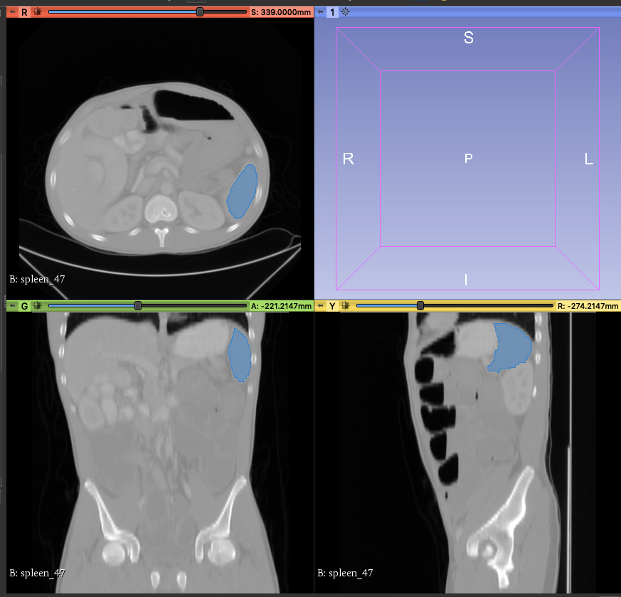:::  4. **Annotation Assistance** At this point, you will see that there are additional areas marked in blue in the CT image, and these blue areas are the results of the spleen location inferred by the model you selected.  ## 5. AIAA Client - Jupyter If you do not have medical image processing software such as **3D Slicer** or OHIF installed, you can use **Jupyter Notebook** to invoke the inference service. ### 5.1 Start Jupyter Notebook This section describes how to use **Container Service** to start Jupyter Notebook. #### 5.1.1 Create Container Service Click **Container Service** from the OneAI service list to enter the container service management page, and click **+CREATE**. 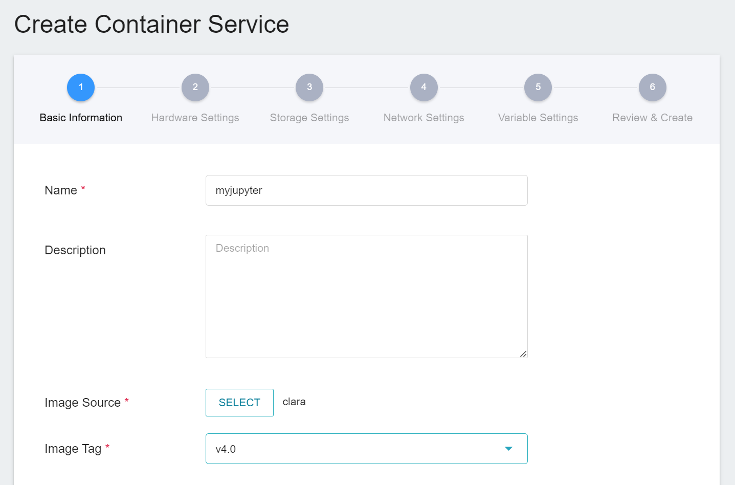1. **Basic Information** When creating a container service, you can directly select the **`clara:v4.0`** image, in which we have provided the relevant environment of Jupyter Notebook.  2. **Hardware Settings** Select the hardware settings. Take into consideration of resource usage when selecting the resources, it is not necessary to configure GPU. 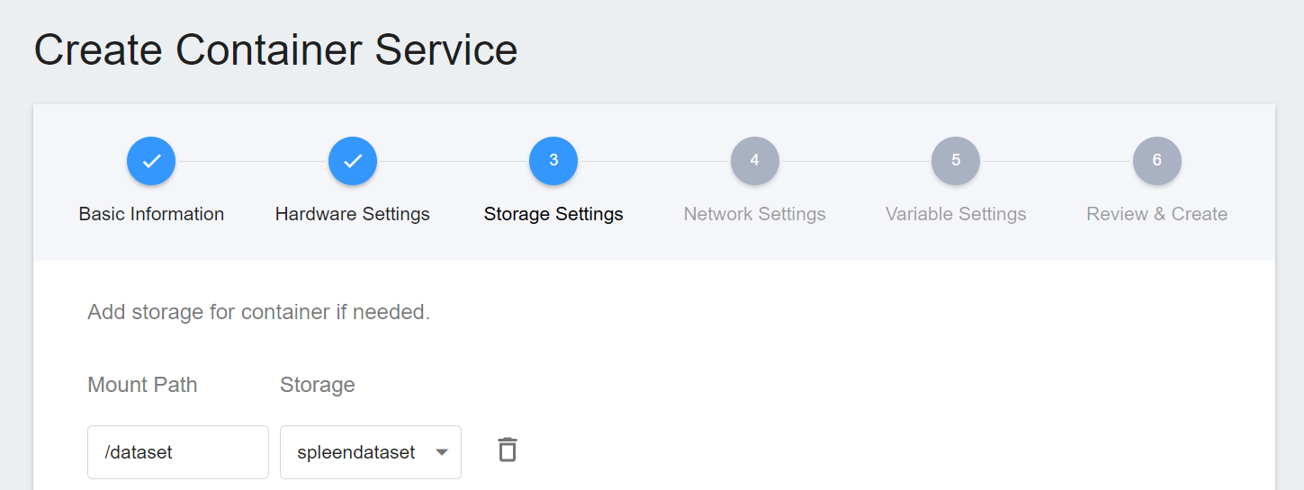3. **Storage Settings** To facilitate the subsequent acquisition of CT images of the spleen for inference, we directly selected the original spleen dataset bucket in the storage step for inference.  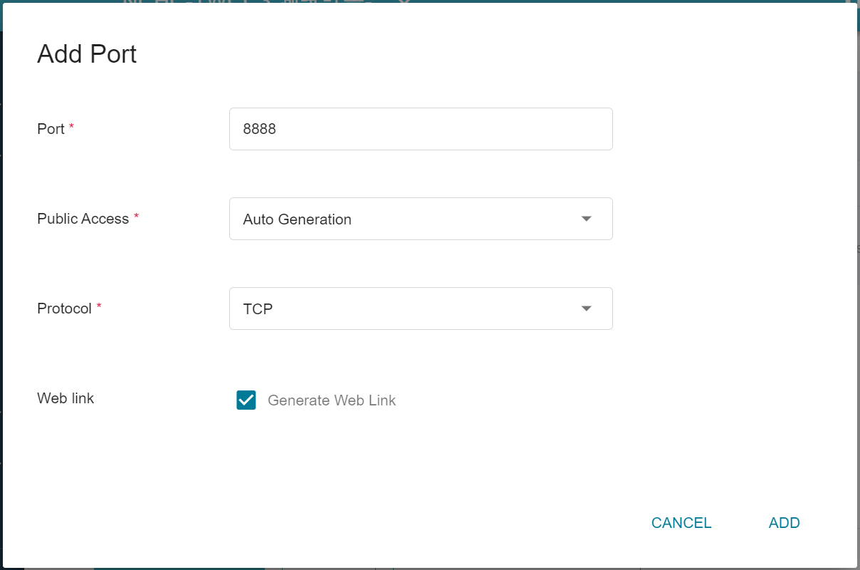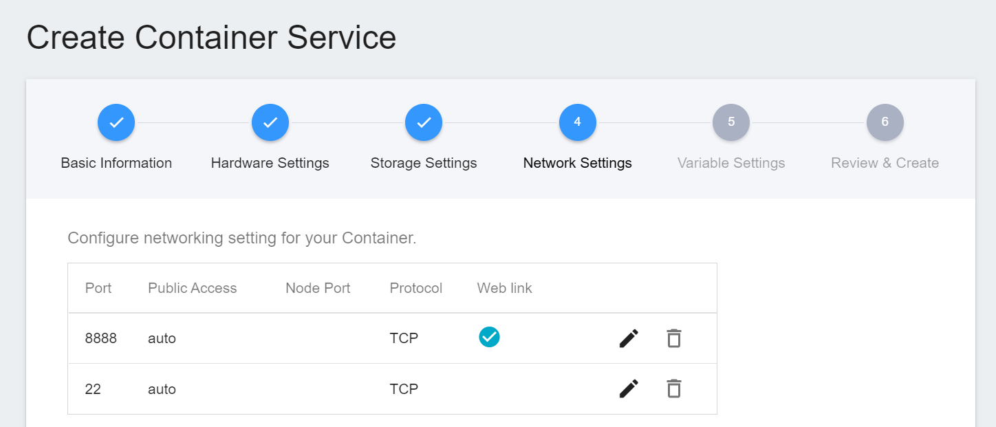4. **Network Settings** The Jupyter Notebook service runs on port 8888 by default. In order to access Jupyter Notebook from the outside, you need to set up an external public service port. For convenience, we also open port 22 used by SSH.   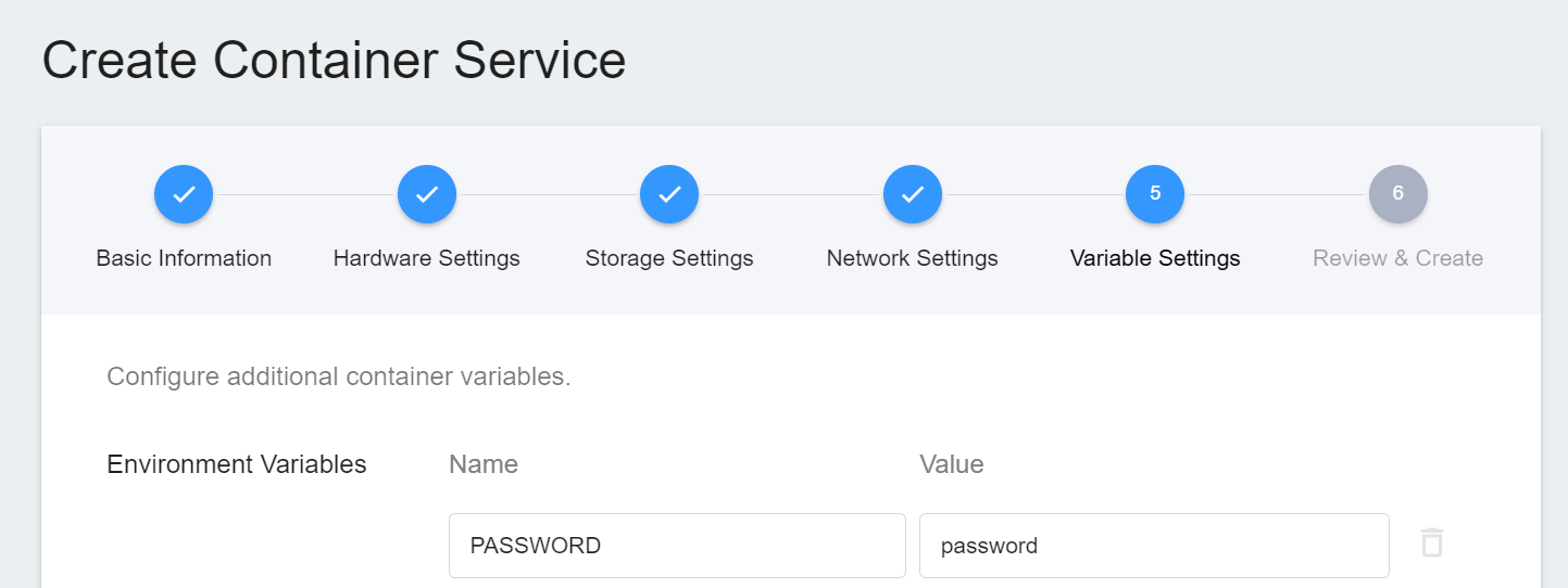5. **Variable Settings** To use Jupyter Notebook, you will need to enter a password. You can use the environment variables for the image to set the password.  6. **Create** Once the above settings are complete, you can finally review and confirm the information, and then click **CREATE**. #### 5.1.2 **Use Jupyter Notebook** After creating the container service, go back to the container service management list page and click on the service to get detailed information.  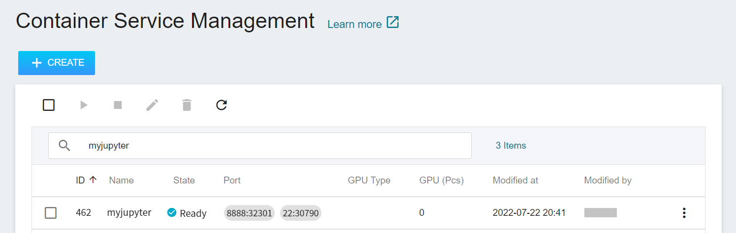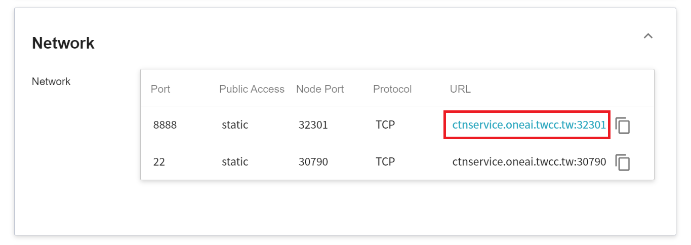In the details page, you should pay special attention to the **Network** section, where there is an external service port `8888` for Jupyter Notebook, click the URL link to open Jupyter Notebook service in your browser.  When the login page of the Jupyter service appears, enter the **`PASSWORD`** variable value set in the **Variable Settings** step.  Now the Jupyter Notebook startup is complete. <br> ### 5.2 Making Inferences If you are using Jupyter Notebook created with Container Service, you can see a program file called `inference.ipynb` in the `inference` folder, and you can make inferences directly from this code. This example is implemented using [**NVIDIA AI-Assisted Annotation Client**](https://github.com/NVIDIA/ai-assisted-annotation-client/tree/71dee28405f58b3d2db001644c480550a9b3f0ba/py_client) provided by NVIDIA. For more information, please refer to the official [**NVIDIA AI-Assisted Annotation Client Documentation**](https://docs.nvidia.com/clara/aiaa/sdk-api/docs/index.html). 1. **AIAA Client object** First use the API to retrieve the constructor of an AIAA Client, which will include some server information. Please change the value of url to the URL obtained in the step [**3.2 Querying Inference Information**](#32-Querying-Inference-Information). :::info :bulb: **Tips:** The URLs in the document are for reference only, and the URLs you got may be different. ::: ```python import client_api #user config url = "http://myinference-i:5000" client = client_api.AIAAClient(server_url=url) ``` <br> For example, use `model_list` to retrieve information about some supported models. ```python models = client.model_list() [{'name': 'mymodel-latest', 'labels': ['spleen'], 'description': 'A pre-trained model for volumetric (3D) segmentation of the spleen from CT image', 'version': '2', 'type': 'segmentation'}] ``` <br> 3. **segmentation** Since the model we trained is suitable for segmentation technology, we have to select `segmentation` when choosing the execution method, and we have to pass in the selected model and image during the call, and specify the medical image, and finally indicate the location where the segmentation result will be written. Pay attention to the model name to be used here. The model name used here is from the environment variables we declared when we created the inference service in Section [**3.2 Querying Inference Information**](#32-Querying-Inference-Information) - **MODEL_NAME** and **MODLE_VERSION**, which are **mymodel** and **latest** respectively. Of course you can also use `model_list` to view this information. 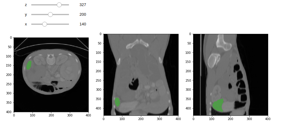```python model_name = "mymodel-latest" image_in = '/dataset/imagesTr/spleen_47.nii.gz' image_out = '/tmp/spleen_inf.nii.gz' client.segmentation( model= model_name, image_in=image_in, image_out=image_out) ``` <br> When the result is retrieved, the image annotation block can be drawn.  <br> ### 5.3 Attached Code 1. :::spoiler **inference.ipynb** ```python=1 import client_api #user config url = "http://myinference-i:5000" client = client_api.AIAAClient(server_url=url) model_name = "mymodel-latest" image_in = '/dataset/imagesTr/spleen_47.nii.gz' image_out = '/tmp/spleen_inf.nii.gz' models = client.model_list() print(models) client.segmentation( model= model_name, image_in=image_in, image_out=image_out) %matplotlib inline import matplotlib.pyplot as plt import SimpleITK as sitk from myshow import myshow, myshow3d rawImage = sitk.ReadImage(image_in) # Read image annotation file anoImage = sitk.ReadImage(image_out) # Convert image to 8-bit unsigned integer rawImageUint8 = sitk.Cast(sitk.RescaleIntensity(rawImage, outputMinimum=0, outputMaximum=255), sitk.sitkUInt8) # Overlay annotation images overlay = sitk.LabelOverlay(rawImageUint8, anoImage, opacity=0.4) myshow(overlay) ``` ::: 2. :::spoiler **myshow.ipynb** ```python=1 import SimpleITK as sitk import matplotlib.pyplot as plt from ipywidgets import interact, interactive from ipywidgets import widgets def myshow(img, title=None, margin=0.05, dpi=80 ): nda = sitk.GetArrayFromImage(img) spacing = img.GetSpacing() slicer = False if nda.ndim == 3: # fastest dim, either component or x c = nda.shape[-1] # the the number of components is 3 or 4 consider it an RGB image if not c in (3,4): slicer = True elif nda.ndim == 4: c = nda.shape[-1] if not c in (3,4): raise RuntimeError("Unable to show 3D-vector Image") # take a z-slice slicer = True if (slicer): ysize = nda.shape[1] xsize = nda.shape[2] else: ysize = nda.shape[0] xsize = nda.shape[1] # Make a figure big enough to accomodate an axis of xpixels by ypixels # as well as the ticklabels, etc... figsize = (1 + margin) * ysize / dpi, (1 + margin) * xsize / dpi def mycallback(z=None,y=None,x=None): fig, axs = plt.subplots(1, 3, figsize=(15, 5)) plt.set_cmap("gray") axs[0].imshow(nda[z,:,:],interpolation=None) axs[1].imshow(nda[:,y,:],interpolation=None) axs[2].imshow(nda[:,:,x],interpolation=None) plt.show() def callback(z=None,y=None,x=None): extent = (0, xsize*spacing[1], ysize*spacing[0], 0) fig = plt.figure(figsize=figsize, dpi=dpi) # Make the axis the right size... ax = fig.add_axes([margin, margin, 1 - 2*margin, 1 - 2*margin]) plt.set_cmap("gray") if z is None: ax.imshow(nda,extent=extent,interpolation=None) else: ax.imshow(nda[z,...],extent=extent,interpolation=None) if title: plt.title(title) plt.show() if slicer: interact(mycallback, z=(0,nda.shape[0]-1),y=(0,nda.shape[1]-1),x=(0,nda.shape[2]-1)) else: callback() def myshow3d(img, xslices=[], yslices=[], zslices=[], title=None, margin=0.05, dpi=80): size = img.GetSize() img_xslices = [img[s,:,:] for s in xslices] img_yslices = [img[:,s,:] for s in yslices] img_zslices = [img[:,:,s] for s in zslices] maxlen = max(len(img_xslices), len(img_yslices), len(img_zslices)) img_null = sitk.Image([0,0], img.GetPixelID(), img.GetNumberOfComponentsPerPixel()) img_slices = [] d = 0 if len(img_xslices): img_slices += img_xslices + [img_null]*(maxlen-len(img_xslices)) d += 1 if len(img_yslices): img_slices += img_yslices + [img_null]*(maxlen-len(img_yslices)) d += 1 if len(img_zslices): img_slices += img_zslices + [img_null]*(maxlen-len(img_zslices)) d +=1 if maxlen != 0: if img.GetNumberOfComponentsPerPixel() == 1: img = sitk.Tile(img_slices, [maxlen,d]) #TODO check in code to get Tile Filter working with VectorImages else: img_comps = [] for i in range(0,img.GetNumberOfComponentsPerPixel()): img_slices_c = [sitk.VectorIndexSelectionCast(s, i) for s in img_slices] img_comps.append(sitk.Tile(img_slices_c, [maxlen,d])) img = sitk.Compose(img_comps) myshow(img, title, margin, dpi) ``` ::: 3. :::spoiler **client_api** [Source Code](https://github.com/NVIDIA/ai-assisted-annotation-client/blob/71dee28405f58b3d2db001644c480550a9b3f0ba/py_client/client_api.py) ::: <style> mark { background-color: pink; color: black; } </style>