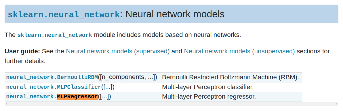
[OneAI Documentation](/s/user-guide-en) # AI Maker Case Study - Machine Learning with Tabular Data: Regression [TOC] ## 0. Introduction In supervised learning, when the predicted target value is non-continuous (ie discrete), it is called **Classification**; if the target value is continuous, it is called **Regression**. | Classification | Regression | | 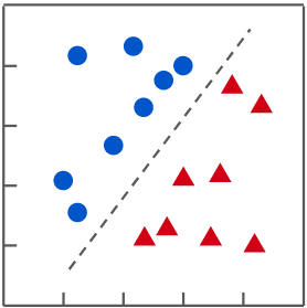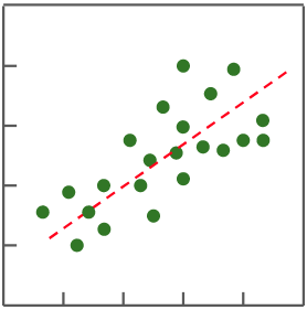:------------------: | :--------------: | |  |  | | In a classification problem, find a function that separates different categories of data | In a regression problem, find a function that fits the distribution of data | In this example, we will use "tabular data" for regression and explanation, and gradually build the machine learning application with tabular data from scratch. The steps are as follows: 1. [**Prepare the Dataset**](#1-Prepare-the-dataset-and-upload) At this stage, we will download the dataset from Kaggle and upload it to the designated location. Currently, Kaggle is the largest data science competition platform. 2. [**Train the Model**](#2-Train-the-Regression-Model) At this stage, we will configure the relevant training job and use specified algorithms to train and fit the model, and store the trained model for inference service. 3. [**Create Inference Service**](#3-Create-Inference-Service) At this stage, we will deploy the stored model and create a web service for the model to perform inference. 4. [**[Advanced Operations] Adjust the Parameters of Algorithm**](#4-Advanced-Operations-Adjust-the-Parameters-of-Algorithm) At this stage, we will learn how to further adjust the algorithm parameters when the machine learning results are not as expected. This tutorial provides a template named **`ml-sklearn-regression`**, you only need to upload the dataset you want to train and configure the environment variables required for training, then you are ready to train and validate. ## 1. Prepare Dataset And Upload ### 1.1 Data Format Description Use **tabular data**, which is two-dimensional data consisting of Columns and Rows, with a **.csv** file extension, as shown in the table below. sample_dataset.csv | | Column 1 | Column 2 | Column 3 | ... | Column 9 | | ----- | -------- | -------- | -------- | --- | -------- | | **Row 1** | A1 | B1 | C1 | | I1 | | **Row 2** | A2 | B2 | C2 | | I2 | | **Row 3** | A2 | B3 | C3 | | I3 | | **...** | | | | | | | **Row 9** | A9 | B9 | C9 | | I9 | The original table data needs to be split into **feature data (file name: train_x.csv)** and **target value data (file name: train_y.csv)** to be used as the input of the training model. - **Feature data (file name: train_x.csv)** It is the known data columns that will be used to predict the target value data. - **Target value data (file name: train_y.csv, only one column of data)** It is the real target value data, which is used for training and comparing with predicted values. :::info :bulb: **Tips: Tools for Splitting Data** Generally, it can be processed quickly through spreadsheet software, such as **Microsoft Excel**, [**Google Sheets**](https://docs.google.com/spreadsheets/) and **LibreOffice Calc**. It can be done by deleting fields and then saving a new file. ::: ### 1.2 Prepare Data This tutorial uses the public dataset provided by Kaggle: **[house prices data](https://www.kaggle.com/c/house-prices-advanced-regression-techniques/data)** as an example. #### 1.2.1 Data Download Enter from the **Data** tab, you can see **train.csv** and **test.csv** (no target value data), which can be downloaded separately.  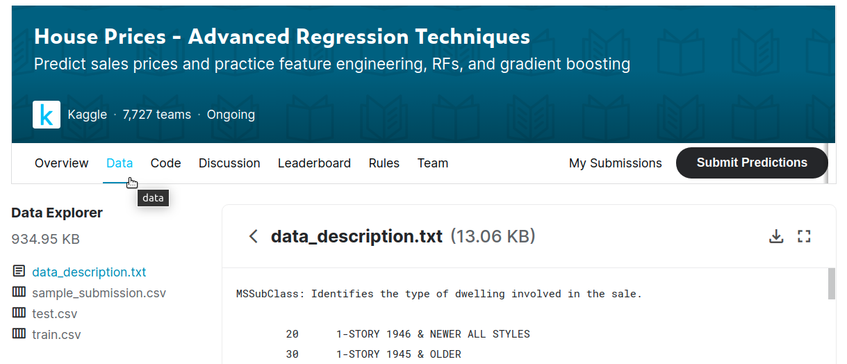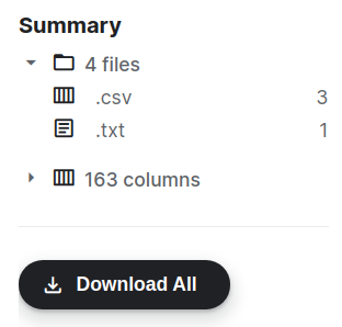Scroll to the page bottom, you can see the **`Download All`** button, click this button to download all the data.  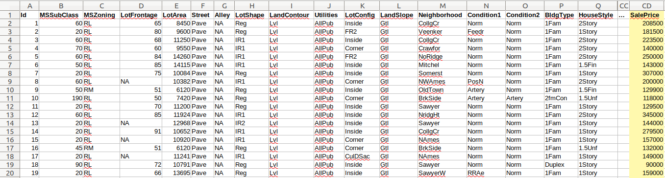#### 1.2.2 Data Disassembly In a regression task, as show in the example below, whether it is a sample dataset or a custom dataset, the dataset will contain two types of information: 1. **Feature (Feature Data)**: Information such as house type, year of construction, roof type, basement condition, street type...etc. 2. **Regression Result (Target Value Data)**: Such as house **SalePrice**. Follow the steps below to re-split the dataset and convert the dataset into a format acceptable for model training: - **train.csv (1460 data rows, 81 columns or fields)** The last column (field), **SalePrice**, is the target variable to be predicted. We split train.csv into: - train_x.csv (without SalePrice field) - train_x.csv (with only SalePrice field) - **test.csv (1459 data rows, 80 columns)** Since test.csv contains no target value data, we renamed test.csv to test_x.csv. There is no test_y.csv for this example. The final data file is as shown below: | | Features | Regression Result | | ------------- | ----------- | ----------- | |train.csv | train_x.csv | train_y.csv | | test.csv | test_x.csv | - | Next, prepare to upload the two files: train_x.csv and train_y.csv. 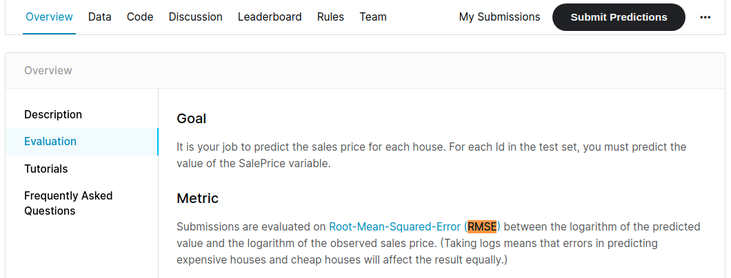Finally, we will use the local test dataset **test_x.csv** as the test, and upload the prediction result **test_y.csv** to the Kaggle platform for comparison. The Kaggle platform will use the **RMSE (Root-Mean-Squared-Error)** evaluation metric to score the regression results.  #### 1.2.3 Column Description For column (field) descriptions, please refer to: - [**Online Description**](https://www.kaggle.com/c/house-prices-advanced-regression-techniques/data) (only field description) - The downloaded file data_description.txt contains: - Description of each field - The meaning of the code in the category field #### 1.2.4 Data Content (Example)  ### 1.3 Create A Bucket Once the data is ready, you can go to **Storage Service** service to upload the dataset. 1. **Go to **Storage Service** Service** and Select **Storage Service** from the OneAI service list, enter the Storage Service management page. 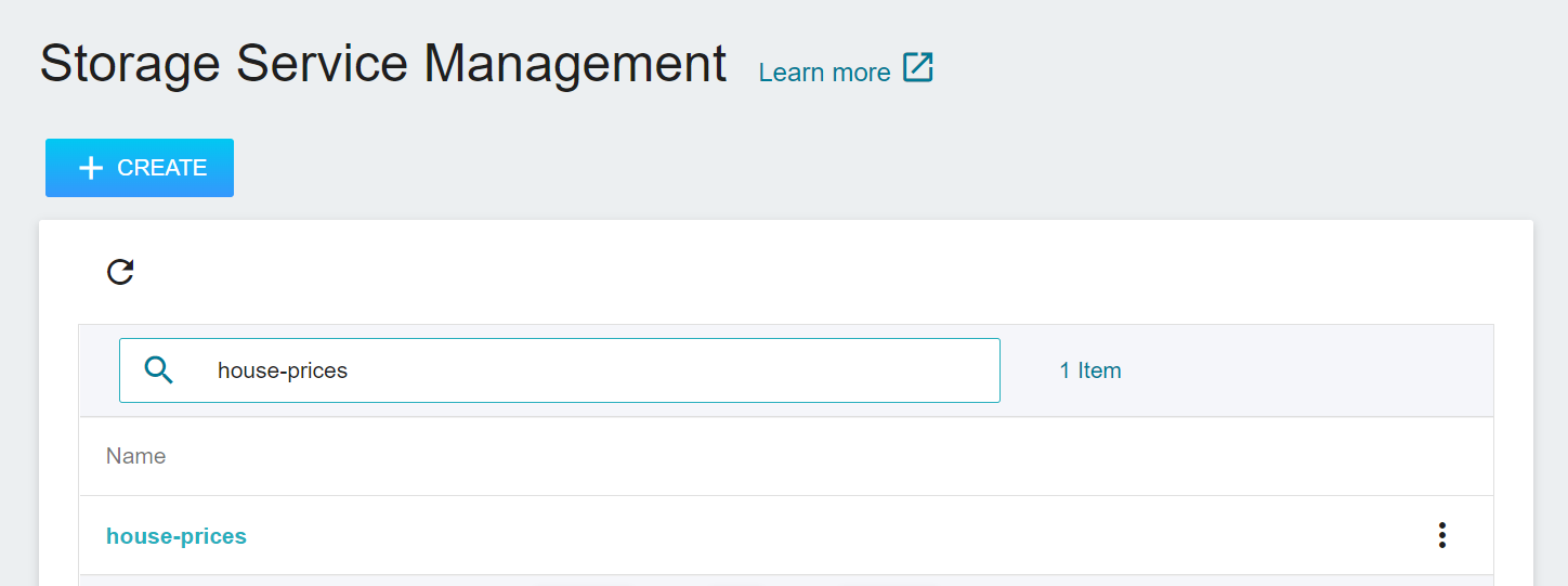2. **Create A Bucket** Then click **+CREATE** to add a bucket named **`house-prices`** to store the dataset for training. 3. **View Bucket** After the bucket is created, go back to the Storage Service Management page, click the **`penguin`** bucket justed created and get ready to upload the dataset.  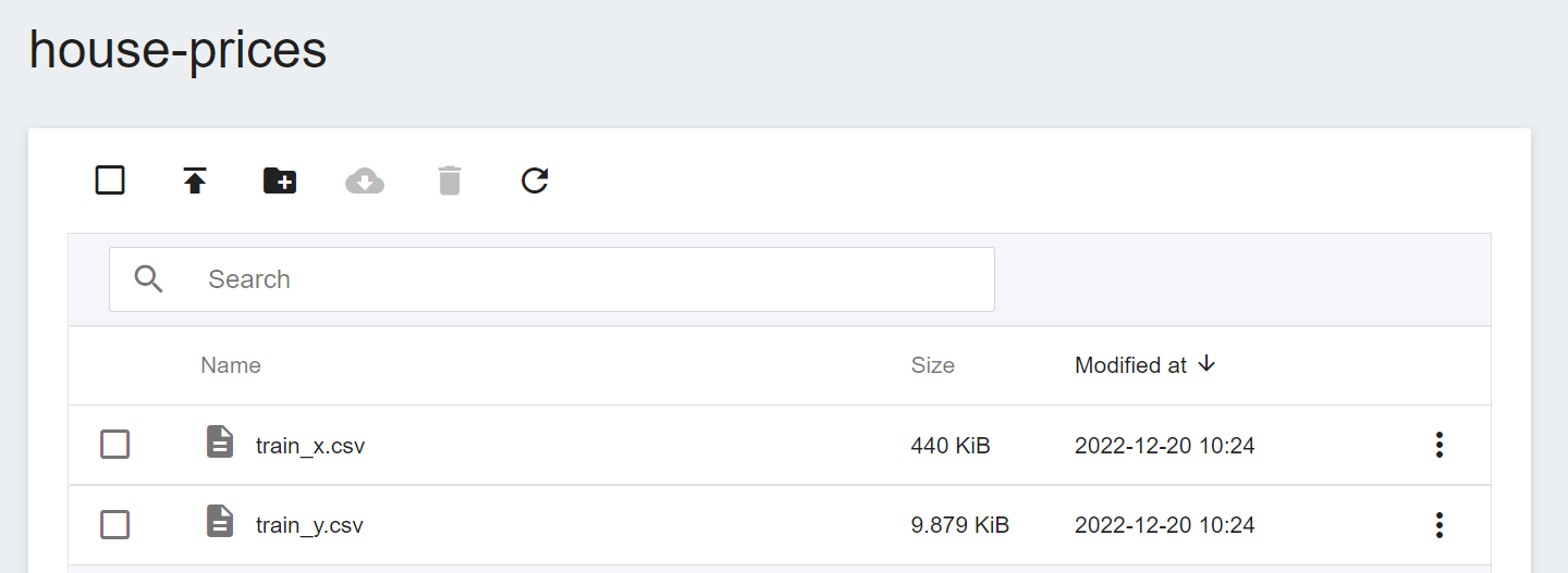### 1.4 Upload Dataset After the bucket is completed, you can start uploading the two house price dataset files train_x.csv and train_y.csv. The results after uploading are as follows:  ## 2. Train the Regression Model After completing the [**Upload Dataset**](#1-Prepare-Dataset-And-Upload), you can use these data to train and fit our regression model. 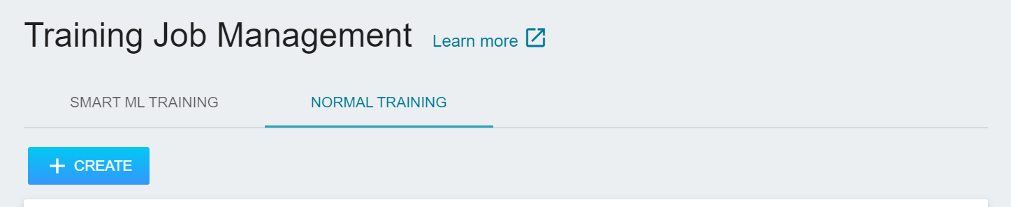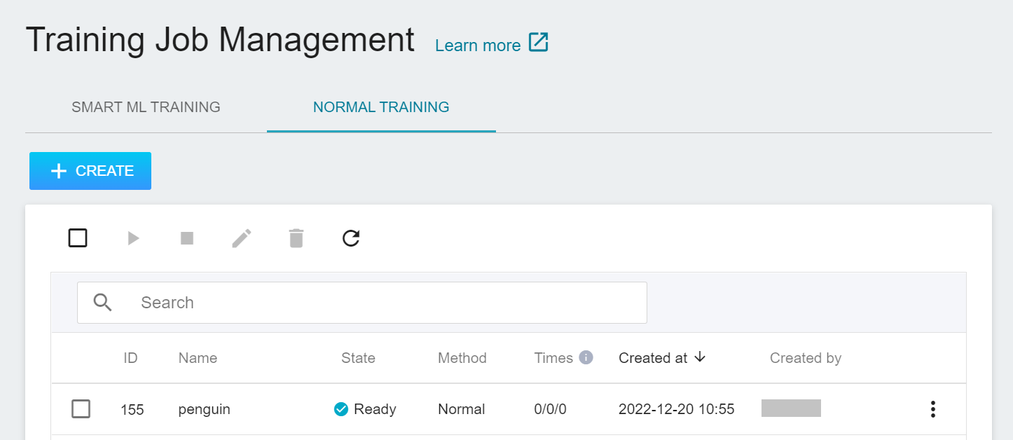### 2.1 Create Training Jobs Select **AI Maker** from the OneAI service list, and then click **Training Jobs**. After entering the training job management page, switch to **Normal Training Jobs** tab, then click **+CREATE** to add a training job.  There are five steps in creating a training job. For detailed instructions, please refer to the [**AI Maker User Manual**](/s/ai-maker-en). 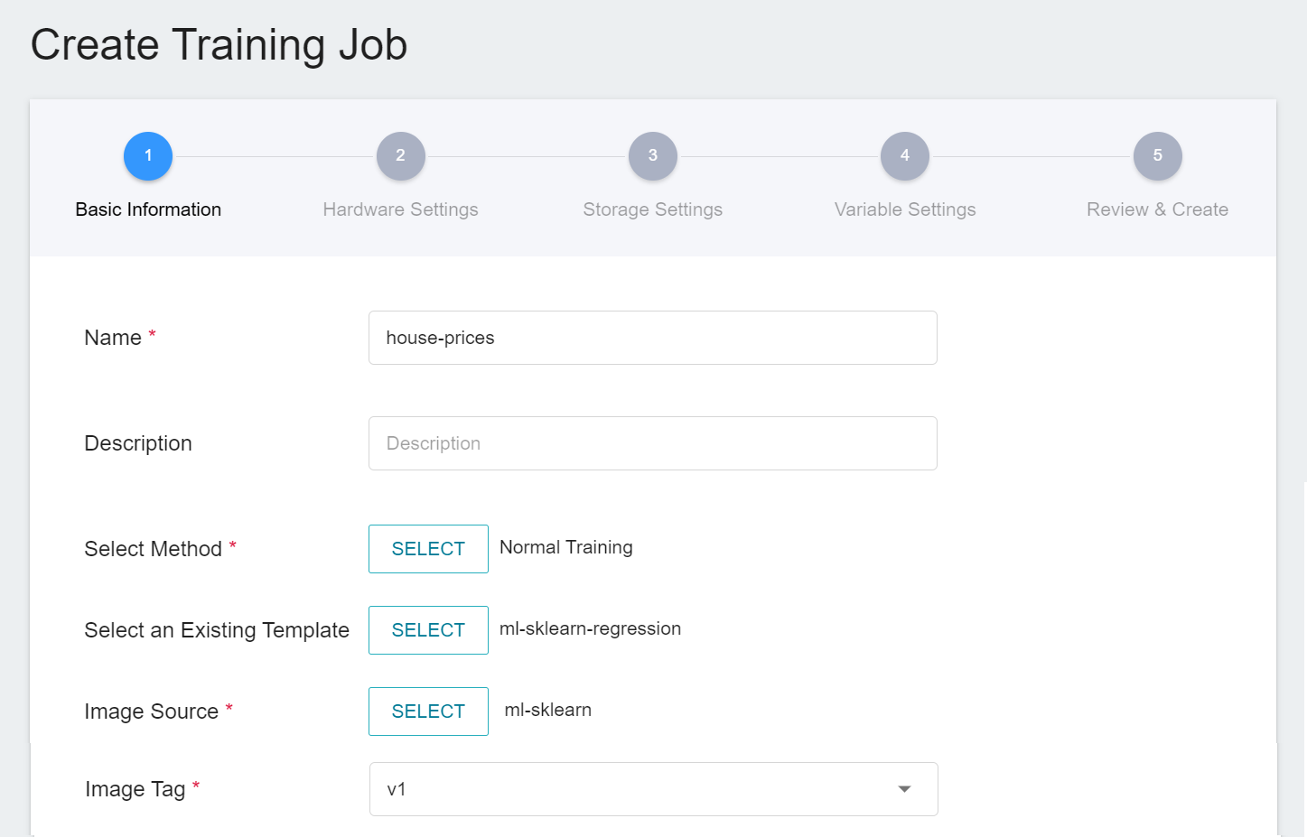#### 2.1.1 Basic Information The first step is to set the basic information, enter the name, description, selection method in sequence, and select the **`ml-sklearn-regression`** template. The template will automatically bring in the public image **`ml-sklearn:v1`** and various parameter settings for subsequent steps.  :::info :bulb: **Tips: Template Feature** AI Maker provides templates that define the default parameters and settings to be used for each stage of the task. You can use the template to quickly apply the parameters or settings to be used for each task to facilitate the workflow and training environment for machine learning. ::: #### 2.1.2 Hardware Settings The machine learning algorithm used in this example can use CPU or GPU computing resources. Please select the appropriate hardware resources from the list according to the current available quota and computing requirements. 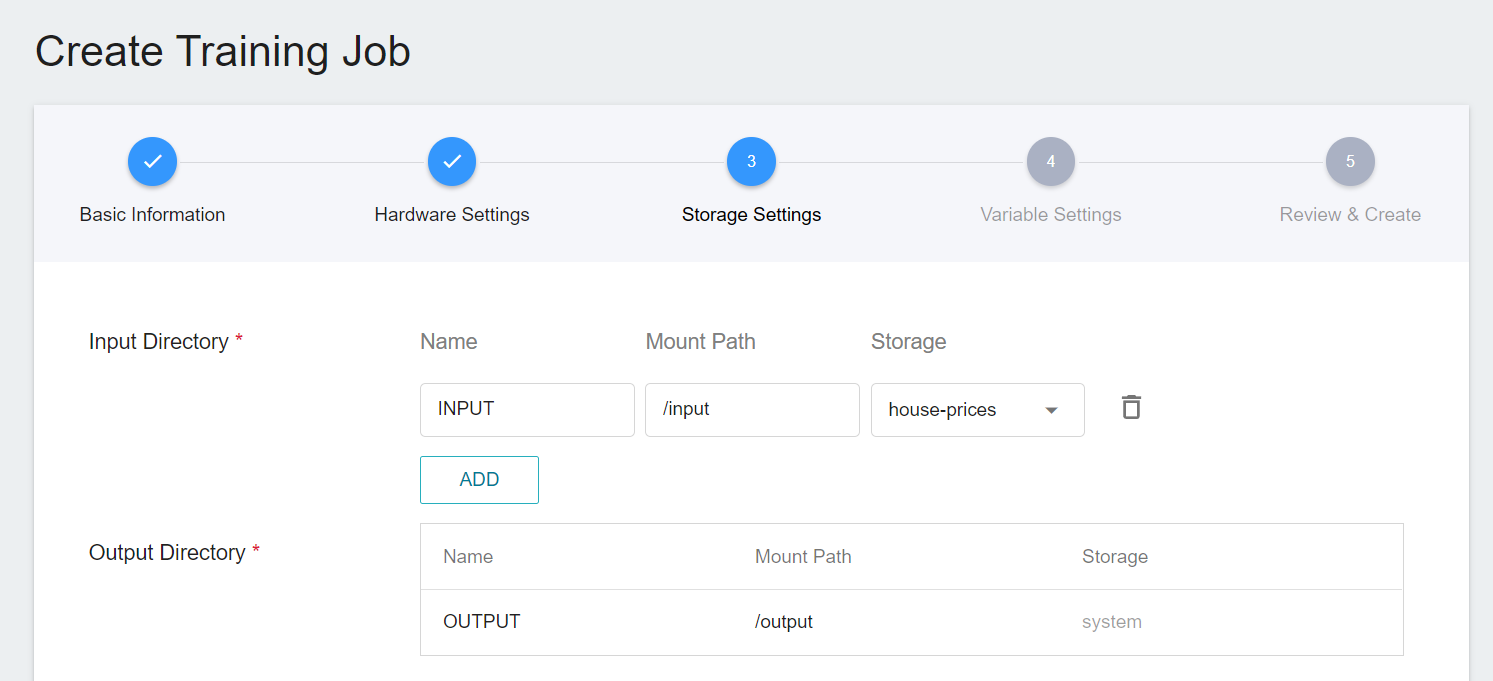#### 2.1.3 Storage Settings The bucket **`house-price`** onto which you previously uploaded dataset needs to be mounted in this step.  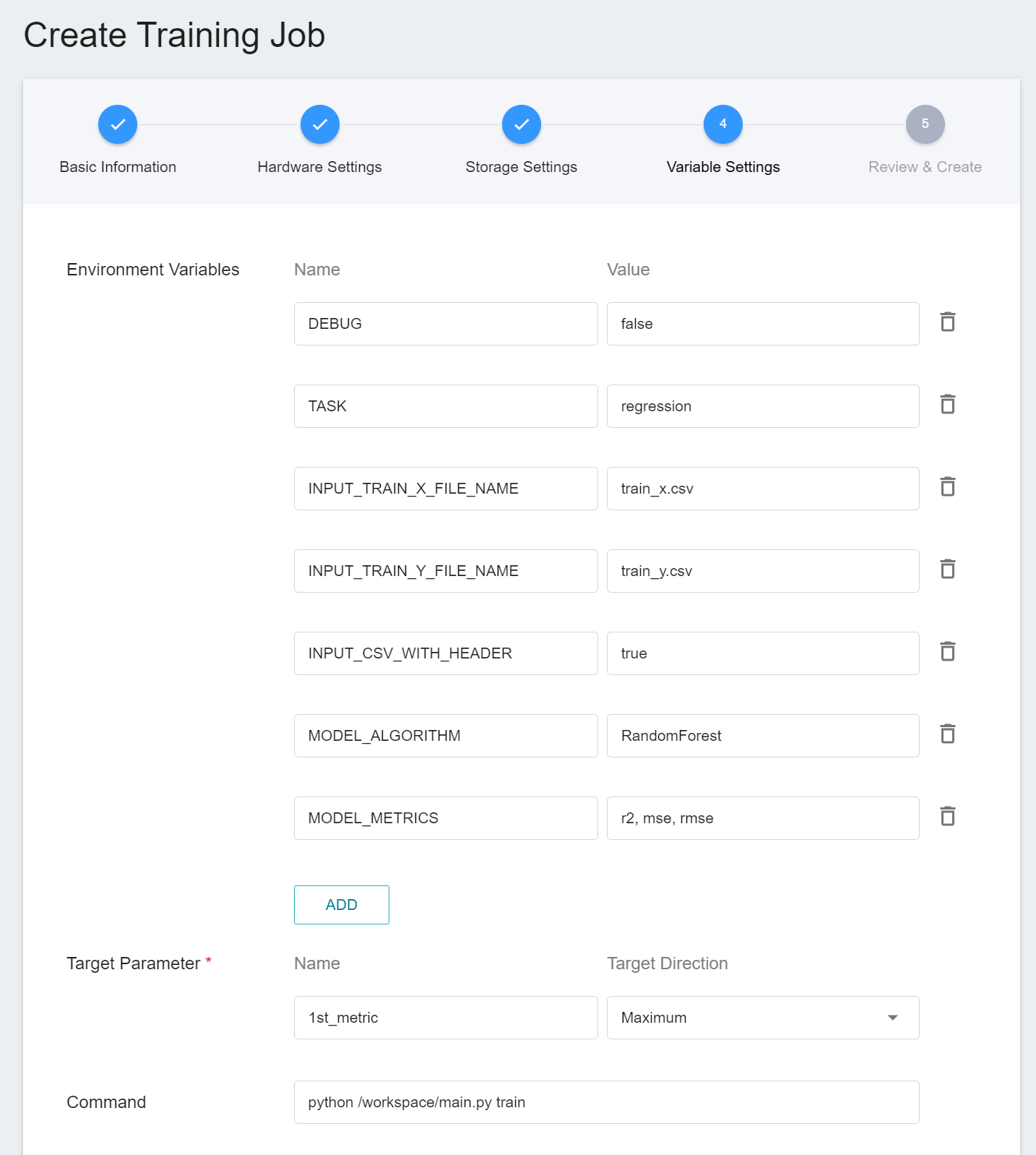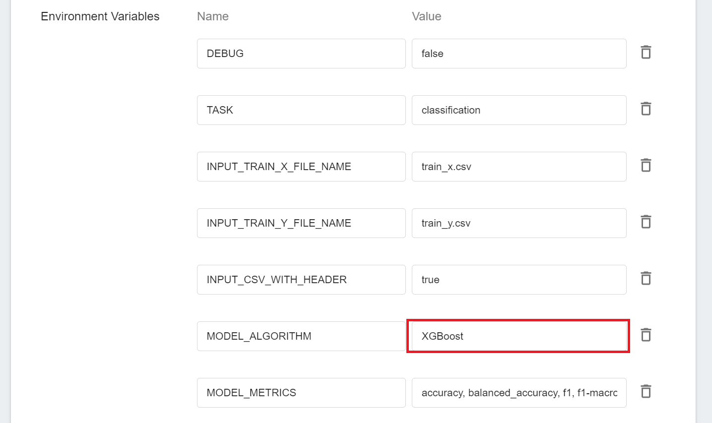#### 2.1.4 Variable Settings Next, set the environment variables and commands. When you choose to use the **`ml-sklearn-regression`** template while entering the basic information, the following variables and settings will be brought in automatically. The parameters are described below, and can be adjusted according to the requirements.  |Parameter |Default |Introduction| |---|-----|---| | [DEBUG](#DEBUG) | `false` | Whether to enable more logs to see the details of machine learning in action. To enable, set the value to `true`; otherwise, set the value to `false`. | | [TASK](#TASK) <sup style="color:red"><b>*</b></sup> | `regression` | The type of tasks that machine learning is going to handle. Set the value to **`classification`** when the problem to be addressed by machine learning is a **classification problem**; set this value to **`regression`** for a **regression problem**.<br>| | INPUT_TRAIN_X_FILE_NAME | `train_x.csv` | The file name of the feature data to be trained. | | INPUT_TRAIN_Y_FILE_NAME | `train_y.csv` | The file name of the regression result to be trained. | | <span style="white-space: nowrap">[INPUT_CSV_WITH_HEADER](#INPUT_CSV_WITH_HEADER) <sup style="color:red"><b>*</b></sup></span> | `true` | If the dataset to be trained has a field name, set the value to `true`; if not, set the value to `false`. | | [MODEL_ALGORITHM](#MODEL_ALGORITHM) <sup style="color:red"><b>*</b></sup> | `RandomForest` | Algorithm used in machine learning. | | [MODEL_METRICS](#MODEL_METRICS) | `r2, mse, rmse` | Various metrics used to evaluate the the regression model, please use `,` (comma) to separate each one, currently limited to log output. | <sup style="color:red"><b>\*</b></sup> In general, the parameters that need to be noted when using machine learning are **TASK**, **INPUT_CSV_WITH_HEADER** and **MODEL_ALGORITHM**, more details of the parameters are as follows. - #### DEBUG Whether to enable more logs to view details of machine learning in action, including: input and output information for files, column and header information for data tables, information on how much memory is used in data tables, feature processing, and multiple evaluation metrics for models. | Value | Description | | -- | -------- | | `true`<br>`1` | Enable more logs (recommended) | | The rest of the values | Disable logs | - #### TASK The type of tasks that machine learning is going to handle. | Value | Description | | -- | -------- | | `regression` | Machine learning will use the **regression** algorithm, see [**`MODEL_ALGORITHM`**](#MODEL_ALGORITHM) description | | `classification` | Machine learning will use the **classification** algorithm, see [**`MODEL_ALGORITHM`**](#MODEL_ALGORITHM) description | - #### INPUT_CSV_WITH_HEADER Whether the dataset to train has field names. | Value | Description | | -- | -------- | | `true`<br>`1` | Indicates that in the csv file, the first row are the field names | | The rest of the values | Indicates that in the csv file, the first row are not the field names, and are just data | - #### MODEL_ALGORITHM Algorithm used in machine learning. | Value | Support Classification | Support Regression | Additional Note<br>See detailed descriptions below the table | | --------------------- |:--------:|:--------:| -------- | | `Auto` | ✔ | ✔ | Automatic machine learning (Auto-ML) with **automatic algorithm selection** and **hyperparameter adjustment** | | `AutoGluon` | ✔ | ✔ | An AutoML tool that supports CPU & GPU | | `AutoSklearn` | ✔ | ✔ | An AutoML tool that does not support GPU, but can still be executed in a GPU environment | | `AdaBoost` | ✔ | ✔ | Adaptive enhancement | | `ExtraTree` | ✔ | ✔ | Extremely randomized tree | | `DecisionTree` | ✔ | ✔ | Decision tree | | <span style="white-space: nowrap">`GradientBoosting`</span> | ✔ | ✔ | Gradient boosting | | `KNeighbors` | ✔ | ✔ | k nearest neighbors | | `LightGBM` | ✔ | ✔ | Efficient gradient boosting decision tree | | <span style="white-space: nowrap">`LinearRegression`</span> | ✘ | ✔ | Linear regression | | <span style="white-space: nowrap">`LogisticRegression`</span> | ✔ | ✘ | Logistic regression | | `RandomForest` | ✔ | ✔ | Random forest | | `SGD` | ✔ | ✔ | Stochastic gradient descent | | `SVM` | ✔ | ✔ | Support vector machine | | `XGBoost` | ✔ | ✔ | Extreme gradient boosting | :::spoiler **What happens when the value is set to `Auto`** When the machine learning algorithm is set to `Auto`, the programs provided by the `ml-sklearn` image will choose depending on whether there is GPU in the current hardware resource: - If there is GPU in the hardware resource, the AutoML tool [`AutoGluon`](https://auto.gluon.ai/stable/tutorials/tabular_prediction/index.html) will be used; - Onversely, if there is no GPU in the hardware resource, that is, with only CPU, the AutoML tool [`AutoSklearn`](https://automl.github.io/auto-sklearn/master/index.html) will be used. - In practice, users can also choose to use either [`AutoGluon`](https://auto.gluon.ai/stable/tutorials/tabular_prediction/index.html) or [`AutoSklearn`](https://automl.github.io/auto-sklearn/master/index.html).<br><br> ::: :::spoiler **What happens when the value is set to `AutoGluon`** - The programs provided by the `ml-sklearn` image directly use the `AutoGluon` set of AutoML tools. - By default, `AutoGluon` integrates the underlying machine learning algorithms during training and produces a more powerful model. | Algorithm name | Support GPU | Documentation | | -------- | ------ | ---- | | CatBoost | ✔ | [View](https://catboost.ai/) | | ExtraTrees | | [View](https://scikit-learn.org/stable/modules/generated/sklearn.ensemble.ExtraTreesClassifier.html) | | KNeightbors | | [View](https://scikit-learn.org/stable/modules/generated/sklearn.neighbors.KNeighborsClassifier.html) | | LightGBM | | [View](https://lightgbm.readthedocs.io/en/latest/) | | NeuralNetFast | ✔ | [View](https://docs.fast.ai/tabular.models.html) | | NeuralNetTorch | ✔ | - | | RandomForest | | [View](https://scikit-learn.org/stable/modules/generated/sklearn.ensemble.RandomForestClassifier.html) | | XGBoost | ✔ | [View](https://xgboost.readthedocs.io/en/latest/) | - `AutoGluon` enables GPU mode by default. In the GPU environment, if the algorithm supports GPU, it will use GPU acceleration; if it does not support GPU, it will use CPU for computing. If the user selects `AutoGluon` in an environment without GPU, the CPU mode will be used. - For more detailed introduction, please refer to the official [**documentation**](https://auto.gluon.ai/stable/tutorials/tabular_prediction/index.html).<br> ::: :::spoiler **What happens when the value is set to `AutoSklearn`** - The programs provided by the `ml-sklearn` image directly use the `AutoSklearn` set of AutoML tools. - `AutoSklearn` does not support GPU, but the tool can also be executed in GPU environment, only that it will not use GPU resources. - For more detailed introduction, please refer to the official [**documentation**](https://automl.github.io/auto-sklearn/master/index.html). ::: :::spoiler **Other machine learning algorithms** <span id="footnote_experimental_algorithm_class_list"></span>If the machine learning algorithm used does not appear in the above list, the user can select it from the list below. Below is a list of all the **values** (in alphabetical order) that can be used by the the regression model algorithm: - `AdaBoostRegressor` - `ARDRegression` - `AutoGluonRegressor` - `AutoSklearnRegressor` - `BaggingRegressor` - `BayesianRidge` - `DecisionTreeRegressor` - `DummyRegressor` - `ExtraTreeRegressor` - `ExtraTreesRegressor` - `GammaRegressor` - `GaussianProcessRegressor` - `GradientBoostingRegressor` - `HuberRegressor` - `KernelRidge` - `KNeighborsRegressor` - `LGBMRegressor` - `LinearRegression` - `LinearSVR` - `MLPRegressor` - `NuSVR` - `PassiveAggressiveRegressor` - `PoissonRegressor` - `RadiusNeighborsRegressor` - `RandomForestRegressor` - `RANSACRegressor` - `Ridge` - `RidgeCV` - `SGDRegressor` - `SVR` - `TheilSenRegressor` - `TransformedTargetRegressor` - `TweedieRegressor` - `XGBRegressor` ::: - #### MODEL_METRICS Various metrics used to evaluate the regression model, please use `,` (comma) to separate each one, currently limited to log output. If this environment variable is not defined, the default evaluation metric will use `r2`. Settings example: - `r2` - `rmse` - `r2, rmse, mse` <br> | Value | Description | | -- | -------- | | `r2` | [Usage description](https://scikit-learn.org/stable/modules/generated/sklearn.metrics.r2_score.html) | | `explained_variance` | [Usage description](https://scikit-learn.org/stable/modules/model_evaluation.html#explained-variance-score) | | `max_error` | [Usage description](https://scikit-learn.org/stable/modules/model_evaluation.html#max-error) | | `neg_mean_absolute_error` | [Usage description](https://scikit-learn.org/stable/modules/model_evaluation.html#mean-absolute-error) | | `neg_mean_squared_error` or `mse` | [Usage description](https://scikit-learn.org/stable/modules/model_evaluation.html#mean-squared-error) | | `neg_root_mean_squared_error` or `rmse` | [Usage description](https://scikit-learn.org/stable/modules/model_evaluation.html#mean-squared-error) | | `neg_mean_squared_log_error` | [Usage description](https://scikit-learn.org/stable/modules/model_evaluation.html#mean-squared-log-error) | | `neg_median_absolute_error` | [Usage description](https://scikit-learn.org/stable/modules/model_evaluation.html#median-absolute-error) | | `neg_mean_poisson_deviance` | [Usage description](https://scikit-learn.org/stable/modules/model_evaluation.html#mean-tweedie-deviance) | | `neg_mean_gamma_deviance` | [Usage description](https://scikit-learn.org/stable/modules/model_evaluation.html#mean-tweedie-deviance) | | `neg_mean_absolute_percentage_error` | [Usage description](https://scikit-learn.org/stable/modules/model_evaluation.html#mean-absolute-percentage-error) | #### 2.1.5 Review & Create Finally, after confirming that the settings information is correct, click **CREATE**. 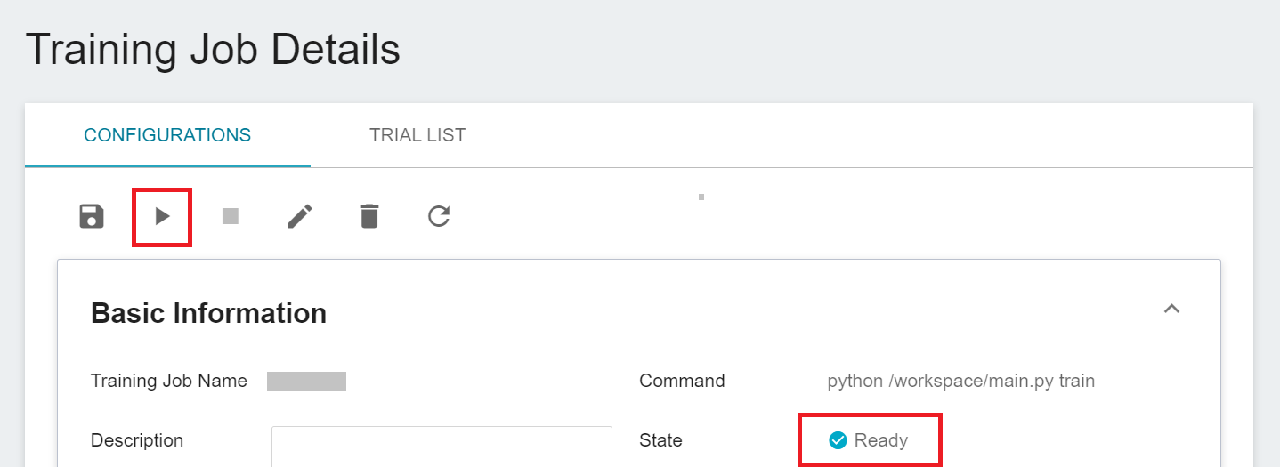### 2.2 Start A Training Job After completing the setting of the training job, go back to the training job management page, and you can see the job you just created. Click the job to view the detailed settings of the training job. If the job state is displayed as **`Ready`** at this time, you can click **START** to execute the training job.   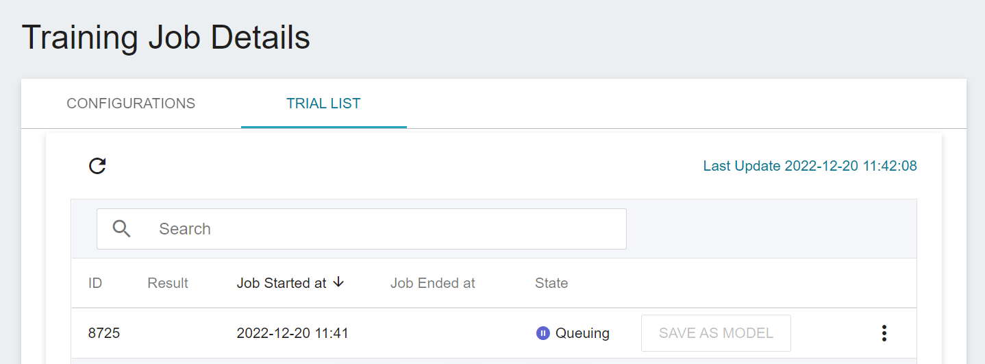Once started, click the **Trial List** tab above to view the execution status and schedule of the job in the list.  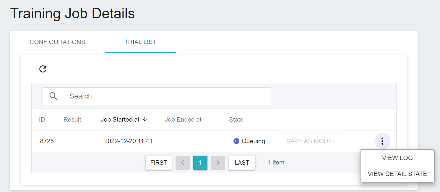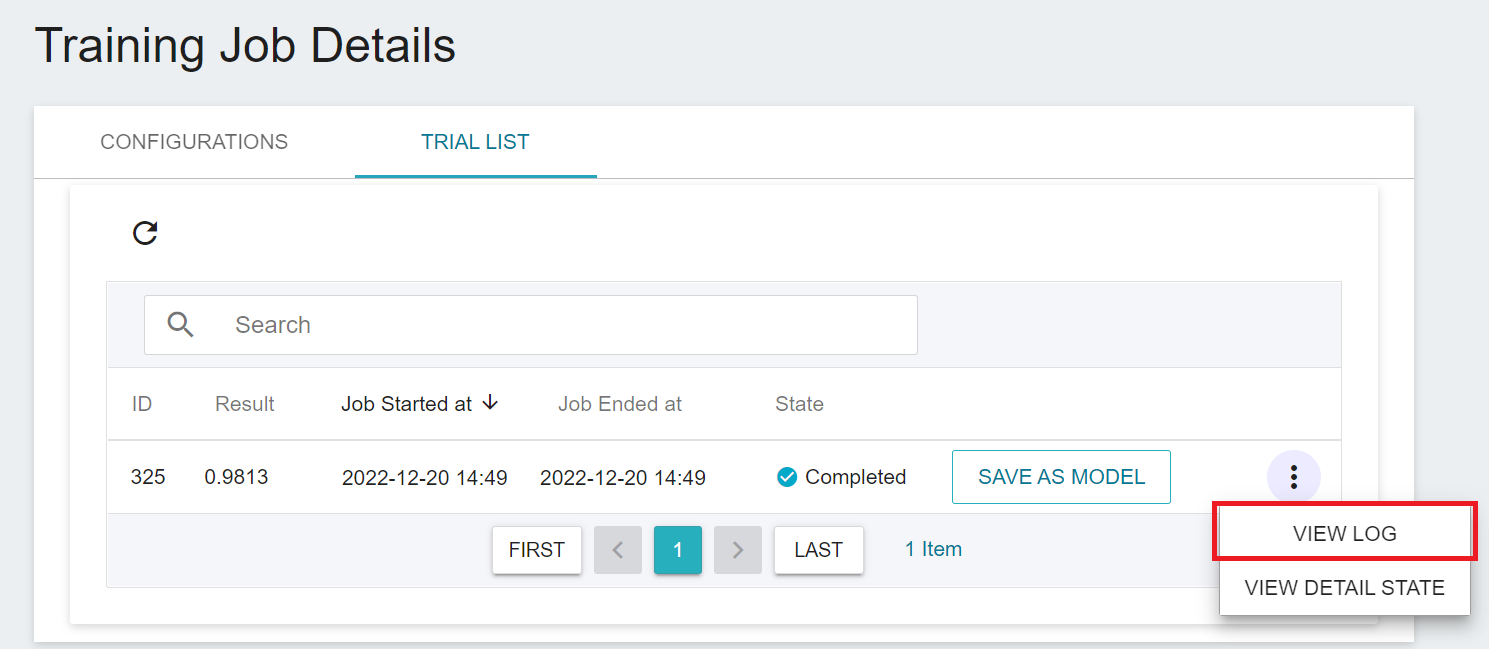During training, you can click **VIEW LOG** or **VIEW DETAIL STATE** in the menu on the right of the job to know the details of the current job execution.  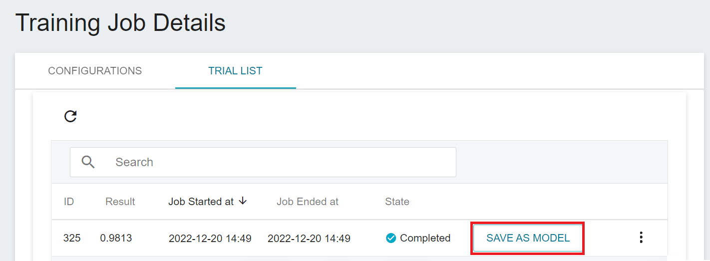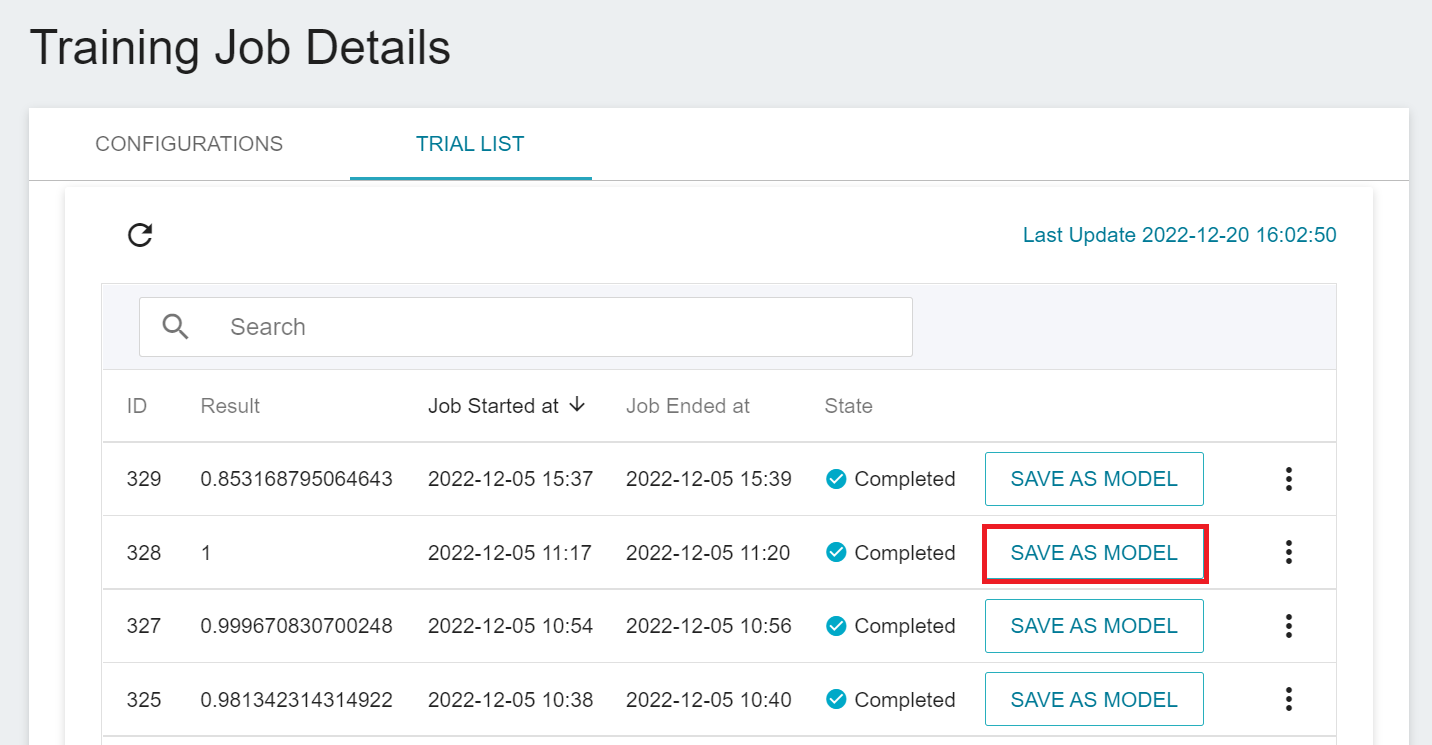### 2.3 View Training Results #### 2.3.1 Model Evaluation Score When the training is complete, the results obtained by the machine learning algorithm **`RandomForest`** used for this task will be displayed. Select the results that meet the expectations, and then click **SAVE AS MODEL** to save them to the **Model Repository**; if no results meet the expected results, Then readjust the value or value range of environment variables and hyperparameters.  You can use the following methods to evaluate the quality of a machine learning model: 1. Use the unseen test dataset (eg: test_x.csv and test_y.csv) to evaluate the model; if there is no test dataset, make atest dataset by subsampling from the training dataset (train_x.csv and train_y.csv). 2. The first metric in the list of metrics set by [**MODEL_METRICS**](#MODEL_METRICS) in the **Environmental Variables** is used as the evaluation metric, refer to the following table: | | MODEL_METRICS Setting Example | Metric Used to Evaluate Result | | ---- | --------------------- | ----------- | | Example 1 | `r2` | `r2` | | Example 2 | `rmse` | `rmse` | | Example 3 | `r2, rmse, mse` | `r2` | | Example 4 | `rmse, mse, r2` | `rmse` | | Example 5 | (No evaluation metric is specified, or the environment variable is not set) | `r2` | #### 2.3.2 Machine Learning Execution Logs Click **View Log** in the menu to the right of the task.  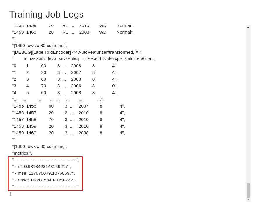Scroll to the bottom of the log to get scores of all evaluation metrics set by [**MODEL_METRICS**](#MODEL_METRICS) in **Environment Variables**.  ### 2.4 Try Different Algorithms And Retrain If the results of the trained model are not as expected, try changing the algorithm and retrain. 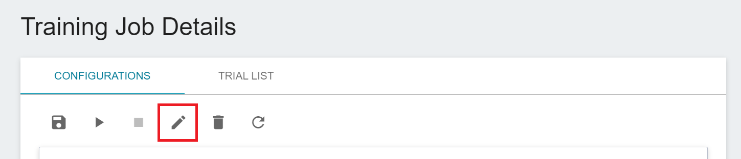1. Click the **CONFIGURATION** tab to return to the configuration page of the training job, and then click **EDIT** on the command bar to modify the settings.  2. Change the [**`MODEL_ALGORITHM`**](#MODEL_ALGORITHM) in the **Environment Variables** to **`XGBoost`**, save it and restart the training job.  After trying different algorithms, go back to the **Trial List** page to see the execution results of multiple jobs.  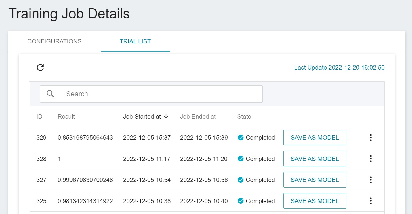| ID | [`MODEL_ALGORITHM`](#MODEL_ALGORITHM) | Model's r2 evaluation score | | ---- | ----------------- | ------ | | 329 | `LinearRegression` | 0.8532 | | 328 | `DecisionTree` | 1.0 | | 327 | `XGBoost` | 0.9997 | | 325 | `RandomForest` | 0.9813 | ### 2.5 Save Model After trying out different algorithms, you can pick the ones that match your expectations and save the model in the **Model Repository**.   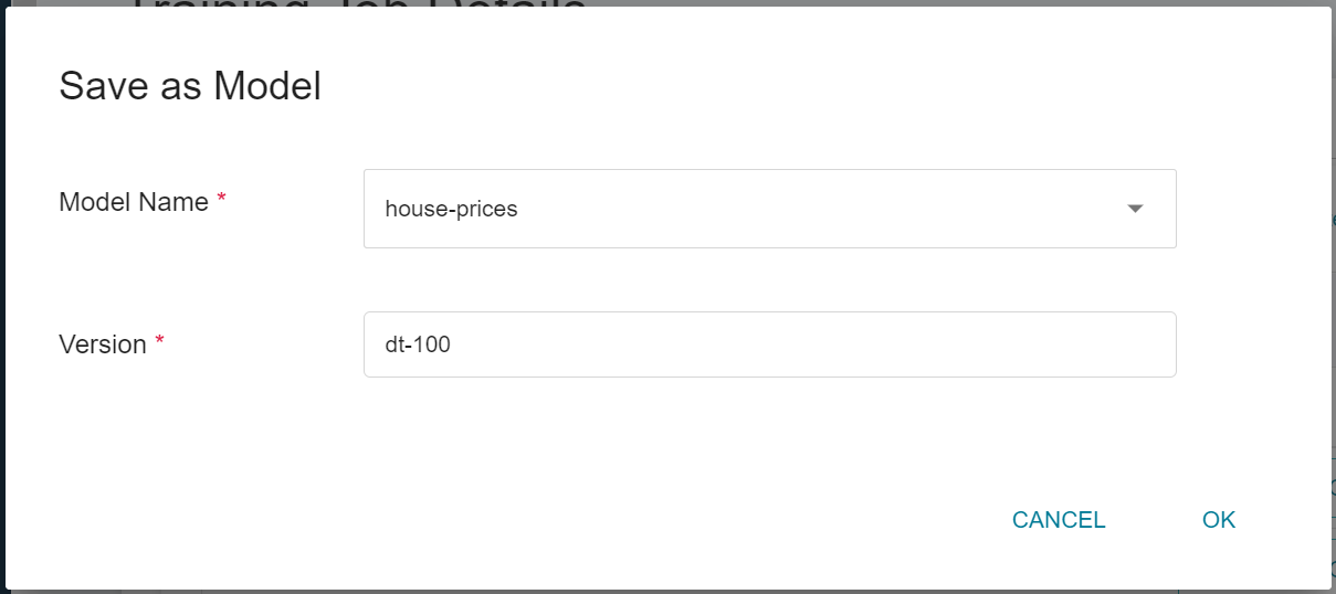Note: `dt-100` is used here to indicate that the model algorithm is `DecisionTree` and its `r2` is 100%. In this example, one or more models can be saved. 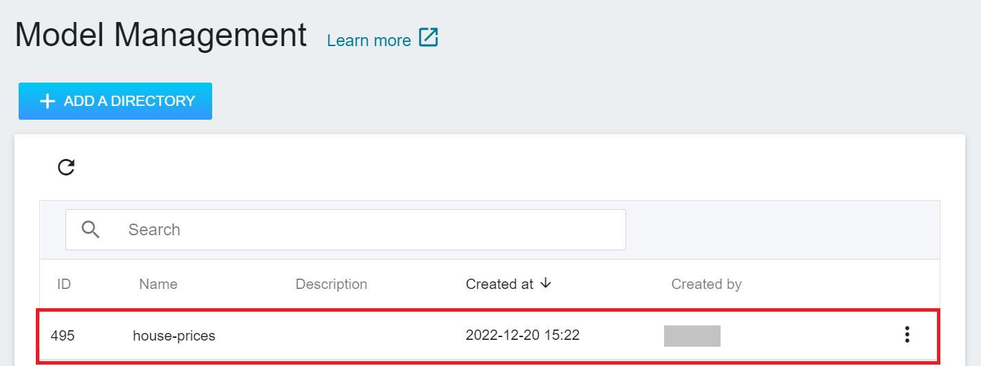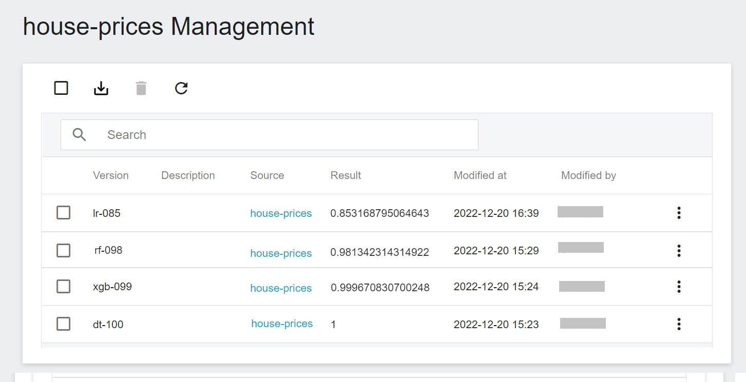| ID | [`MODEL_ALGORITHM`](#MODEL_ALGORITHM) | Model's r2 evaluation score | Model Name | | ---- | ----------------------- | ------ | ------- | | 329 | `LinearRegression` | 0.8532 | `house-prices:lr-085` | | 328 | `DecisionTree` | 1.0 | `house-prices:dt-100` | | 327 | `XGBoost` | 0.9997 | `house-prices:xgb-099` | | 325 | `RandomForest` | 0.9813 | `house-prices:rf-098` | After saving the model, go to the **Model Management** page and click on the `house-prices` directory to find the model in the list of model versions.   ## 3. Create Inference Service Once you have trained the regression model and stored a suitable model, you can then deploy the model as a web service using the **Inference Feature** for an application or service to perform inference. ### 3.1 Create Inference Service Select **AI Maker** from the OneAI service list, then click **Inference** to enter the inference management page, and click **+CREATE** to create an inference service. 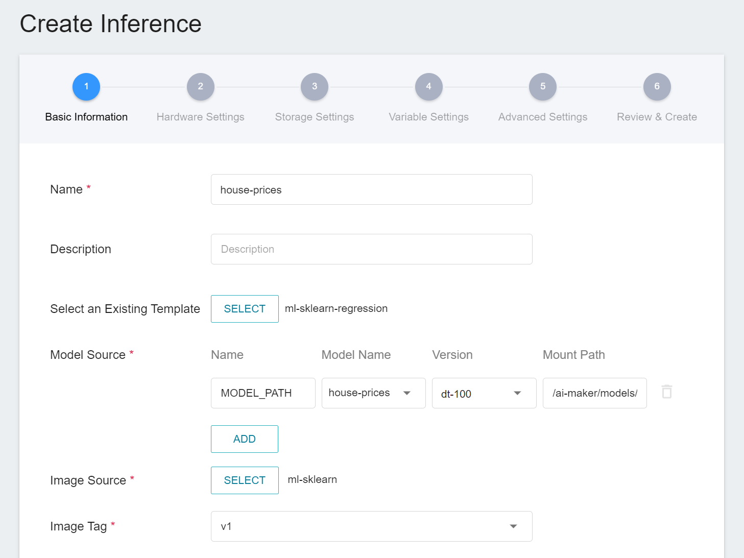The steps for creating the inference service are described below: #### 3.1.1 **Basic Information** Similar to the setting of basic information for training jobs, we also use the **`ml-sklearn-regression`** inference template to facilitate quick setup. The template will automatically bring in the basic settings of the **Source Model**. However, the model name and version number to be loaded still need to be set manually, as shown below.  :::info :bulb: **Tips: Source Model Information** Refer to the model saved in step [**2.5 Save Model**](#25-Save-Model). | ID | [`MODEL_ALGORITHM`](#MODEL_ALGORITHM) | Model's r2 evaluation score | Model Name | | ---- | ----------------------- | ------ | ------- | | 329 | `LinearRegression` | 0.8532 | `house-prices:lr-085` | | 328 | `DecisionTree` | 1.0 | ==`house-prices:dt-100`== | | 327 | `XGBoost` | 0.9997 | `house-prices:xgb-099` | | 325 | `RandomForest` | 0.9813 | `house-prices:rf-098` | ::: #### 3.1.2 **Hardware Settings** Select the appropriate hardware resource from the list with reference to the current available quota and requirements. #### 3.1.3 **Storage Settings** No configuration is required for this step. #### 3.1.4 **Variable Settings** On the Variable Settings page, These commands and parameters are automatically brought in when the template is applied.  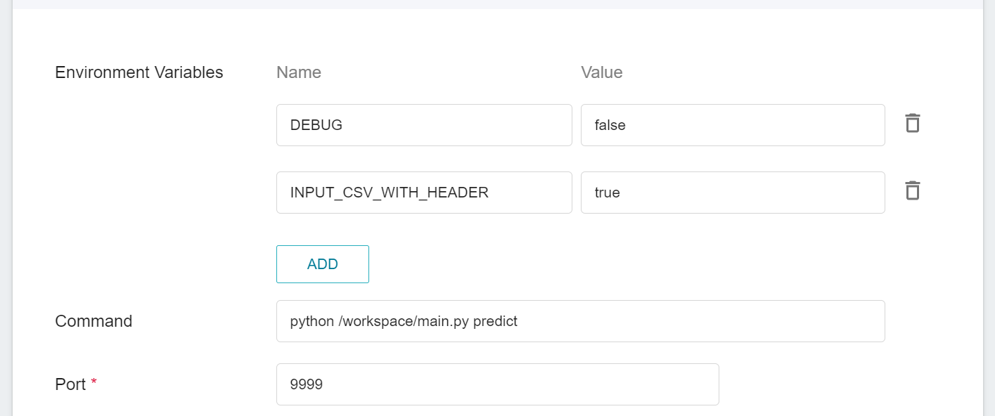The parameters set in **Environment Variables** for this inference template are described as follows: |Parameter |Default |Introduction| |---|-----|---| | [DEBUG](#DEBUG) | `false` | Whether to enable more logs to see the details of inference service. To enable, set the value to `true`; otherwise, set the value to `false`. | | <span style="white-space: nowrap">[INPUT_CSV_WITH_HEADER](#INPUT_CSV_WITH_HEADER) <sup style="color:red"><b>*</b></sup></span> | `true` | If the dataset to be inferred has a field name, set the value to `true`; if not, set the value to `false`. | <sup style="color:red"><b>\*</b></sup> In general, the parameters that need to be noted when using inference are **INPUT_CSV_WITH_HEADER**, more details of the parameters are as follows: - #### `DEBUG` Whether to enable more logs to see the details of inference service. | Value | Description | | -- | -------- | | `true`<br>`1` | Enable more logs (recommended) | | The rest of the values | Disable logs | - #### `INPUT_CSV_WITH_HEADER` Whether the dataset to be inferred has field names. This parameter is used to set the default option of the inference service. Subsequent inference tests do not need to carry this parameter, which simplifies the commands or code required for inference test. | Value | Description | | -- | -------- | | `true`<br>`1` | Indicates that in the csv file, the first row are the field names | | The rest of the values | Indicates that in the csv file, the first row are not the field names, and are just data | #### 3.1.5 Advanced Settings No configuration is required for this step. #### 3.1.6. **Review & Create** Finally, confirm the entered information and click CREATE. 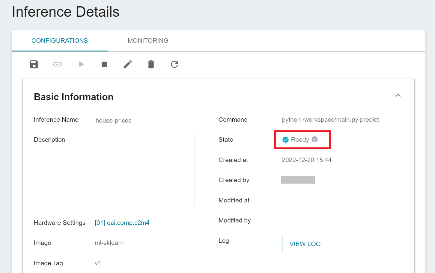### 3.2 Viewing the Status And Endpoint of Inference Service After completing the settings of the inference service, go back to the inference management page, click the inference service you just created to view the basic information. When the service state shows as **`Ready`**, you can start connecting to the inference service for inference.  You can also click **VIEW LOG**. If you see the following message in the log, the inference service is already running.  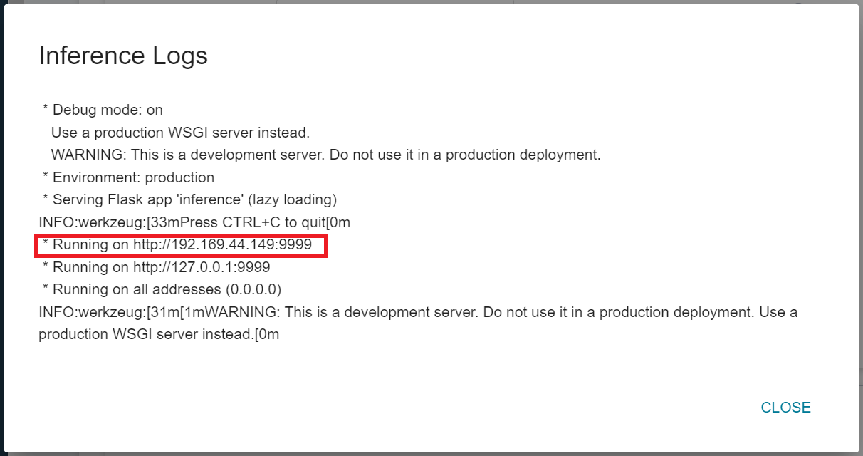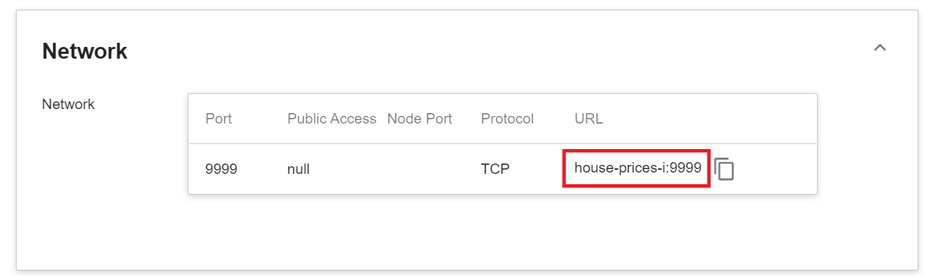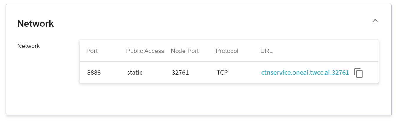Note that the URLhttp://{ip}:{port} displayed in the log is only the internal URL of the container and is not accessible from outside. Since the current inference service does not have a public service port for security reasons, we can communicate with the inference service we created through the Container Service. The way to communicate is through the **Network** Block displayed at the bottom of the **Inference Details** page. :::warning :warning: **Please note:** The URLs in the document are for reference only, and the URLs you got may be different. :::  :::info :bulb: **Tips: Inference Service URL** - For security reasons, the **URL** provided by the inference service can only be used in the system's internal network, and cannot be accessed through the external Internet. - To provide this inference service externally, you need to transfer to the inference service through the [**Container Service**](/s/container-en) for public access. ::: To view inference monitoring, you can click the **Monitoring** tab to see relevant information on the monitoring page. After a period of time, the monitoring page can display the statistics of calls to the inference service API in the past period.  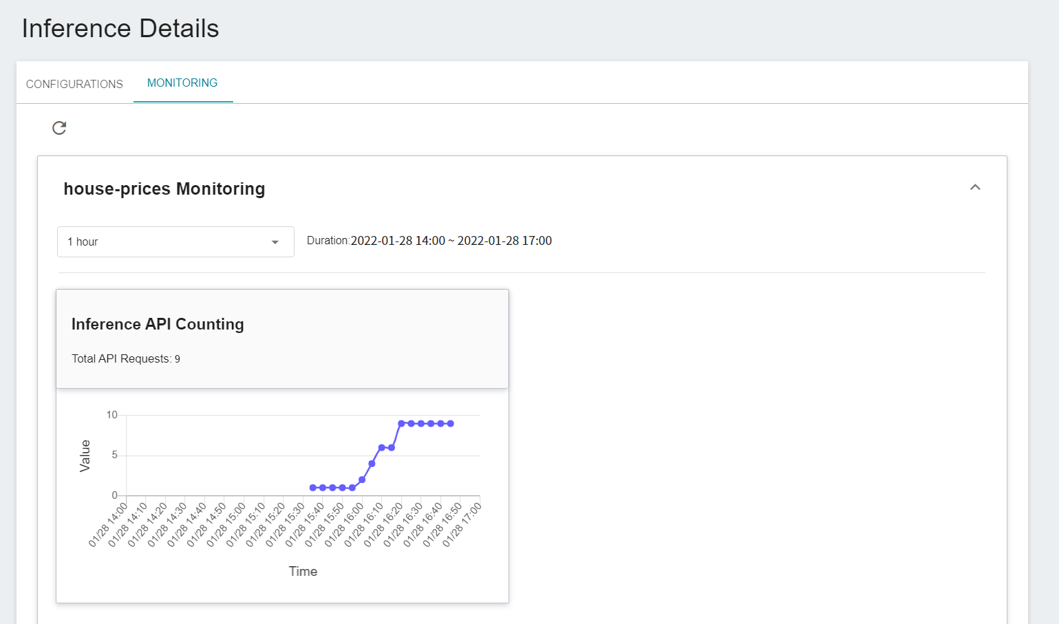Click the Period menu to filter the statistics of the Inference API Call for a specific period, for example: 1 hour, 3 hours, 6 hours, 12 hours, 1 day, 7 days, 14 days, 1 month, 3 months, 6 months, 1 year, or custom.  :::info :bulb: **About the start and end time of the observation period** For example, if the current time is 15:10, then. - **1 Hour** refers to 15:00 ~ 16:00 (not the past hour 14:10 ~ 15:10) - **3 Hours** refers to 13:00 ~ 16:00 - **6 Hours** refers to 10:00 AM ~ 16:00 - And so on. ::: ### 3.3 Start JupyterLab JupyterLab provides a web-based interactive computing environment, users can write programming languages such as Python, R, and more through the web service. Below we will describe how to use the built-in **`ml-sklearn:v1`** image to start the JupyterLab service. 1. Click **Container Service** from the service list to enter the container service management page, and click **+CREATE**. 2. Enter the comtainer name, then select **`ml-sklearn`** image.  3. You can select the most basic hardware resources in the hardware setting step without configuring the GPU. 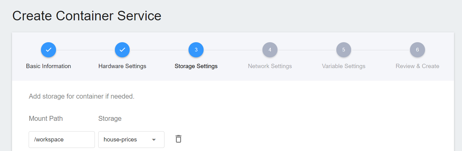4. In the Storage Settings step, set the bucket and mount path for storing the dataset.  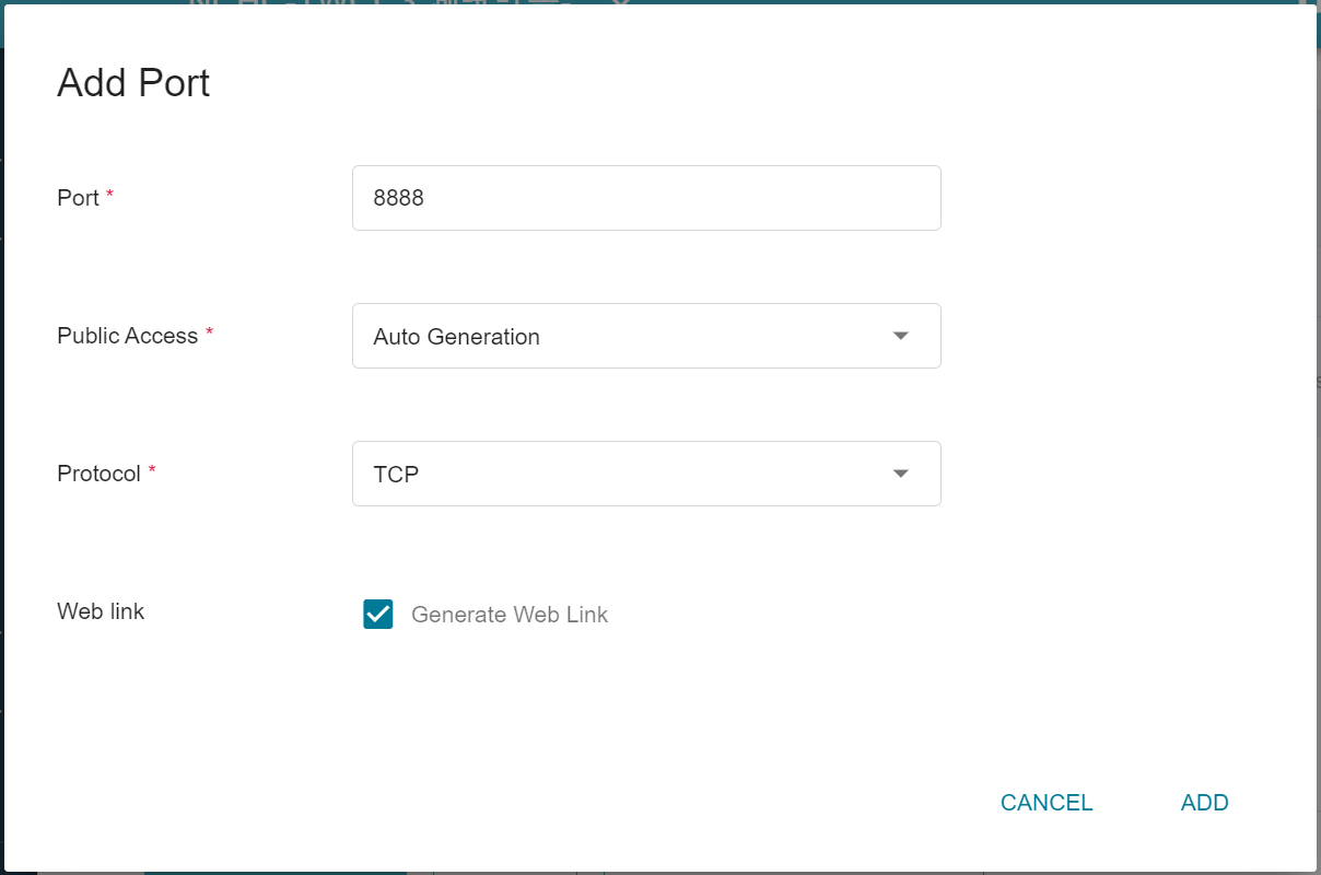5. In order to access this service from the outside, you need to set the connection port of the JupyterLab service to `8888` in the Network Settings step, select the connection port that will automatically generate the external service, and check **Generate Web Link**.  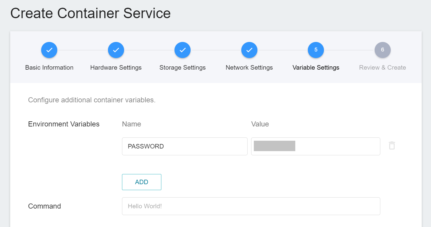6. When using JupyterLab, you will need to enter a password, so in the Variable Settings step, you can use the default environment variable **`PASSWORD`** in the image to set your JupyterLab password.  7. Finally, after checking and confirming that the settings information is correct, click **CREATE**. 8. After the container is successfully created, it will appear in the container service management list. Click the list to view the detailed information of the container. 9. Click the Web link corresponding to port 8888 in the network block to open JupyterLab.  10. Enter your password in JupyterLab's login page and press **Log in** to enter the **Launcher** page.  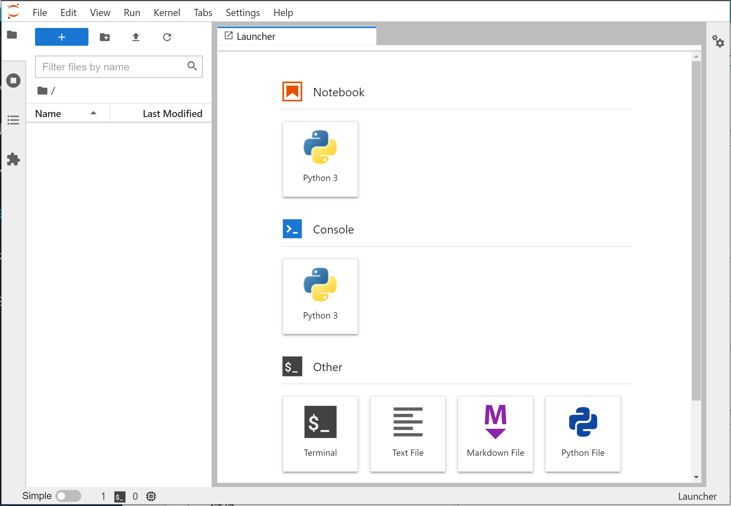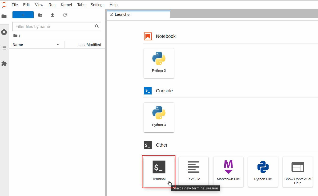### 3.4 Test Inference Service with Curl Command After logging in to JupyterLab, click the **Terminal** icon at the bottom of the **Launcher** page to open the **Terminal**.  Enter the **`curl`** command in the **Terminal** to confirm that the inference service starts normally. ```bash= # "house-prices-i:9999" is the URL for inference service $> curl house-prices-i:9999 Start Inference API! # or $> curl -X GET house-prices-i:9999 Start Inference API! ``` If the service starts successfully, you can call the `predict` API to make inferences. ```bash= $> curl -X POST \ house-prices-i:9999/predict \ -F file=@/house-prices/test_x.csv \ -F INPUT_CSV_WITH_HEADER=true ``` Here: - **`-X POST`** Indicates that the HTTP request method is POST. - **`-F file=@<the location of the dataset on the local side>`** Indicates that the local dataset file is to be uploaded to the inference service for inference; You can use either `train_x.csv` or `test_x.csv` as the dataset file for the test. - **`-F INPUT_CSV_WITH_HEADER=true`** Indicates that in the uploaded dataset, the first row has field names. (Please refer to the description of [**INPUT_CSV_WITH_HEADER**](#INPUT_CSV_WITH_HEADER) variable setting) When the inference service receives the dataset, it will perform predict, and finally return the inference results of the dataset. ```json { "y_pred": [ 129000.0, 130000.0, 192000.0, ... 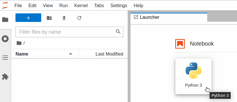137500.0, 105000.0, 219500.0 ] } ``` ### 3.5 Using Python's `requests` Module to Test Inference Service In addition to testing using the Terminal, you can also start the Python environment or the Python Notebook service through the **Container Service**, and test the inference service by executing the following Python code. 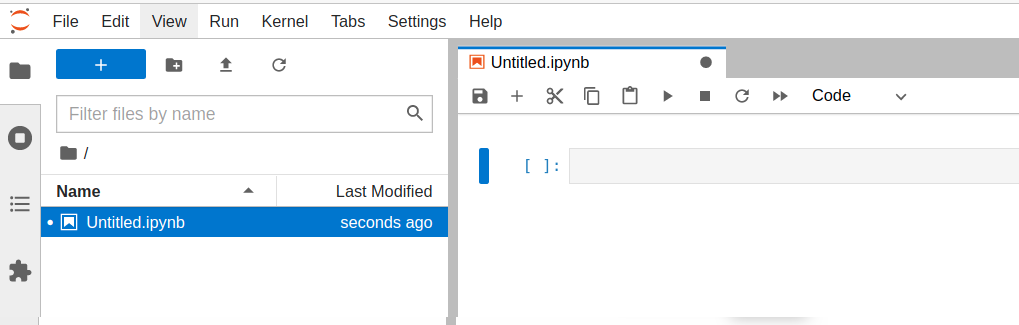Click the **Notebook > Python 3** icon at the top of the JupyterLab Launcher page to open **Notebook**.   Use the **`requests`** module to test online: ```python= import requests import json # prepare the post body my_data = {'INPUT_CSV_WITH_HEADER': True} # read the local dataset my_files = None with open('/house-prices/test_x.csv', 'r') as f: my_files = {'file': f.read()} # send the post request response = requests.post( 'http://house-prices-i:9999/predict', data=my_data, files=my_files) # show the response print('status_code:', response.status_code) print('text:', response.text) print('json:', json.loads(response.text)) ``` Execution result: ``` status_code: 200 text: { "y_pred": [ 129000.0, 130000.0, 192000.0, ... ] } json: {'y_pred': [129000.0, 130000.0, 192000.0, ...]} ``` :::info :bulb: **Note**: Currently there is no `test_y.csv` file. ::: ### 3.6 Upload Results to Kaggle Through Inference Service Since there is no **test_y.csv** file at present, the real target value data is kept by the Kaggle platform. We can refer to the downloaded file **`sample_submission.csv`** in [**1.2.1 Data Download**](#121-Data-Download), the data template is as follows: ```csv Id,SalePrice 1461,169277.0524984 1462,187758.393988768 1463,183583.683569555 ... 2917,219222.423400059 2918,184924.279658997 2919,187741.866657478 ``` From the results of the inference service, the above **`Id`** and **`SalePrice`** field information can be assembled. You can refer to the complete code below: :::spoiler **Complete code** (including: send request, receive response, generate **test_y.csv**) ```python= import os # install related packages (if needed): os.system('pip install requests') os.system('pip install pandas') import requests import json # prepare the post body my_data = {'INPUT_CSV_WITH_HEADER': True} # read the local dataset my_files = None with open('/house-prices/test_x.csv', 'r') as f: my_files = {'file': f.read()} # send the post request response = requests.post( 'http://house-prices-i:9999/predict', data=my_data, files=my_files) # show the response print('status_code:', response.status_code) #print('text:', response.text) #print('json:', json.loads(response.text)['y_pred']) # --- # write the prediction results to the file 'test_y.csv' import pandas df_x = pandas.read_csv('/house-prices/test_x.csv', header=0)['Id'] y_pred = json.loads(response.text)['y_pred'] with open('/house-prices/test_y.csv', 'w') as f: f.write('Id,SalePrice') for idx in range(len(y_pred)): f.write("\n%s,%s" % (df_x.values[idx], y_pred[idx])) # --- print("Next step: upload 'test_y.csv' to Kaggle") ``` ::: <br> Go to the [**upload page**](https://www.kaggle.com/c/house-prices-advanced-regression-techniques/submit) of House Prices and complete the upload in three steps: 1. Upload the **test_y.csv** file 2. Briefly describe the upload, such as: **predicted the house prices via AI Maker/ Decision Tree** 3. 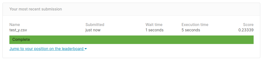Click **Make Submissions** As shown in the example below:  The scoring result will then appear:  This inference resulted in a [**Root-Mean-Squared-Error (RMSE)**](https://www.kaggle.com/c/house-prices-advanced-regression-techniques/overview/evaluation) evaluation score of 0.23339. Click **`Jump to your position on the leaderboard`** to see your ranking. :::info :bulb: **Tips: Try to use other registered models and compare the results** Refer to the model saved in step [**2.5 Save Model**](#25-Save-Model). | ID | [`MODEL_ALGORITHM`](#MODEL_ALGORITHM) | Model's r2 evaluation score | Model Name | Kaggle's RMSE evaluation score | | ---- | ----------------------- | ------ | ------- | ----- | 329 | `LinearRegression` | 0.8532 | `house-prices:lr-085` |0.45732 | | 328 | `DecisionTree` | 1.0 | `house-prices:dt-100` | 0.23339 | | 327 | `XGBoost` | 0.9997 | `house-prices:xgb-099` | 0.14806 | | 325 | `RandomForest` | 0.9813 | `house-prices:rf-098` | 0.14654 | ::: :::info :bulb: **Tips: Continuously improve inference results** In addition to generating additional features through **Feature Engineering**, algorithms can also be used. [**`MODEL_ALGORITHM`**](#MODEL_ALGORITHM) can optionally use the `Auto` option if costs such as time and money are not considered. For detailed usage, please refer to the setting in next section [**4-3-1**](#431-If-you-want-to-spend-more-time-finding-the-optimal-algorithm-and-hyperparameters-you-need-to-increase-the-calculation-time). The table below shows the detailed evaluation metrics after training with the above algorithm. | MODEL_ALGORITHM | r2 | mse | rmse | Kaggle's RMSE evaluation score | | ------------------- | ------ | ---: | ----: | --------------------- | | `LinearRegression` | 0.8532 | 926033367.3 | 30430.8 | 0.45732 | | `DecisionTree` | 1.0 | 0.0 | 0.0 | 0.23339 | | `XGBoost` | 0.9997 | 2076001.2 | 1440.8 | 0.14806 | | `RandomForest` | 0.9813 | 117670079.1 | 10847.6 | 0.14654 | | `Auto` (executes 24 hours)| 0.9643 | 225401086.1 | 15013.4 | ==0.12742== :+1: | ::: ## 4. [Advanced Operations] Adjust the Parameters of Algorithm :::info :bulb:**Tips:** This section is for advanced operations. If the machine learning result does not meet the expectation and you want to further set or adjust the algorithm parameters, you can refer to the description here. ::: Section [**2.1.4 Variable Settings**](#214-Variable-Settings) has mentioned the [**Algorithm (MODEL_ALGORITHM)**](#MODEL_ALGORITHM) to be used for machine learning. When the default parameters of the algorithm or the training results do not meet the actual requirements, for example: 1. If you want to spend more time finding the optimal algorithm and hyperparameters, you need to increase the calculation time. 2. The number of iterations is not enough, and the model cannot be fit and finalized, and the number of iterations needs to be increased. 3. There are different calculation methods in a single algorithm, and you want to choose different calculation methods to fit the data. 4. To use a polynomial-based algorithm which can increase the complexity of the model by changing the power (exponential part). 5. Change the penalty level (penalty points)...etc. Based on needs, parameters can be adjusted to meet actual requirements. The parameter adjustment is also known as hyerparameter adjustment (tuning). ### 4.1 Parameter Adjustment Method On the [**Variable Settings**](#214-Variable-Settings) page, add one or more sets of key values to change the default parameters of the model algorithm. ### 4.2 Parameter Syntax Rule The rule for setting the algorithm parameters is: the entered [**MODEL_ALGORITHM**](#MODEL_ALGORITHM) value, plus the **parameter name** and **parameter value**. Template: ``` {MODEL_ALGORITHM}_param_{parameter name}: {parameter value} ``` :::info :pencil: **Example 1** - Algorithm name: `AutoSklearn` - Parameter 1 - Name: `time_left_for_this_task` - Value: `60*5` (total execution time, limited to 5 minutes) - Parameter 2 - Name: `per_run_time_limit` - Value: `30` (single test time, limited to 30 Sec)<br><br> After applying the above template, it becomes: ``` AutoSklearn_param_time_left_for_this_task: 60*5 AutoSklearn_param_per_run_time_limit: 30 ``` And set it as an environment variable:  ::: :::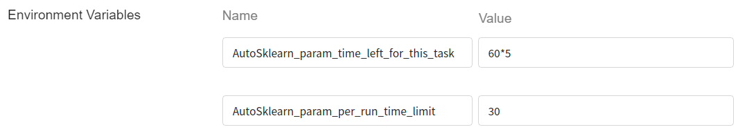info :pencil: **Example 2** - Algorithm category: `AutoSklearnRegressor` - Parameter 1 - Name: `time_left_for_this_task` - Value: `60*5` (total execution time, limited to 5 minutes) - Parameter 2 - Name: `per_run_time_limit` - Value: `30` (single test time, limited to 30 Sec)<br><br> After applying the above template, it becomes: ``` AutoSklearnRegressor_param_time_left_for_this_task: 60*5 AutoSklearnRegressor_param_per_run_time_limit: 30 ``` And set it as an environment variable:  ::: 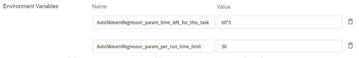The **name** of each algorithm, and its corresponding **class** and **parameter description** are listed below: | Algorithm name | Algorithm category | Parameter description<br>(parameter name & parameter value) | | --------------------- | -------- | -------- | | `Auto` | [^Note 1^](#footnote_auto_algorithm_class) | - | | `AutoSklearn` | AutoSklearnRegressor | [View parameter](https://automl.github.io/auto-sklearn/master/api.html#regression) | | `AutoGluon` | AutoGluonRegressor | View parameter: [init](https://auto.gluon.ai/0.1.0/api/autogluon.task.html#autogluon.tabular.TabularPredictor), [fit](https://auto.gluon.ai/0.1.0/api/autogluon.task.html#autogluon.tabular.TabularPredictor.fit) [^Note 2^](#footnote_autogluon_parameters) | | `AdaBoost` | AdaBoostRegressor | [View parameter](https://scikit-learn.org/stable/modules/generated/sklearn.ensemble.AdaBoostRegressor.html) | | `ExtraTree` | ExtraTreeRegressor | [View parameter](https://scikit-learn.org/stable/modules/generated/sklearn.tree.ExtraTreeRegressor.html) | | `DecisionTree` | DecisionTreeRegressor | [View parameter](https://scikit-learn.org/stable/modules/generated/sklearn.tree.DecisionTreeRegressor.html) | | <span style="white-space: nowrap">`GradientBoosting`</span> | GradientBoostingRegressor | [View parameter](https://scikit-learn.org/stable/modules/generated/sklearn.ensemble.GradientBoostingRegressor.html) | | `KNeighbors` | KNeighborsRegressor | [View parameter](https://scikit-learn.org/stable/modules/generated/sklearn.neighbors.KNeighborsRegressor.html) | | `LightGBM` | LGBMRegressor | [View parameter](https://lightgbm.readthedocs.io/en/latest/pythonapi/lightgbm.LGBMRegressor.html) | | <span style="white-space: nowrap">`LinearRegression`</span> | LinearRegression | [View parameter](https://scikit-learn.org/stable/modules/generated/sklearn.linear_model.LinearRegression.html) | | `RandomForest` | RandomForestRegressor | [View parameter](https://scikit-learn.org/stable/modules/generated/sklearn.ensemble.RandomForestRegressor.html) | | `SGD` | SGDRegressor | [View parameter](https://scikit-learn.org/stable/modules/generated/sklearn.linear_model.SGDRegressor.html) | | `SVM` | SVR | [View parameter](https://scikit-learn.org/stable/modules/generated/sklearn.svm.SVR.html) | | `XGBoost` | XGBRegressor | [View parameter](https://xgboost.readthedocs.io/en/latest/python/python_api.html#xgboost.XGBRegressor) | - <span id="footnote_auto_algorithm_class"></span>**Note 1**: Not recommended, users need to know whether `Auto` is dynamically bound to `AutoSklearnRegressor` or `AutoGluonRegressor` during execution? - Without GPU environment, `Auto` is bound to `AutoSklearnRegressor` - With GPU environment, `Auto` is bound to `AutoGluonRegressor` - <span id="footnote_autogluon_parameters"></span>**Note 2**: AutoGluon currently uses preset parameters. - There are two sources of parameters for adjustment: - One source is [init parameter](https://auto.gluon.ai/0.1.0/api/autogluon.task.html#autogluon.tabular.TabularPredictor); - Another source is [fit parameter](https://auto.gluon.ai/0.1.0/api/autogluon.task.html#autogluon.tabular.TabularPredictor.fit). 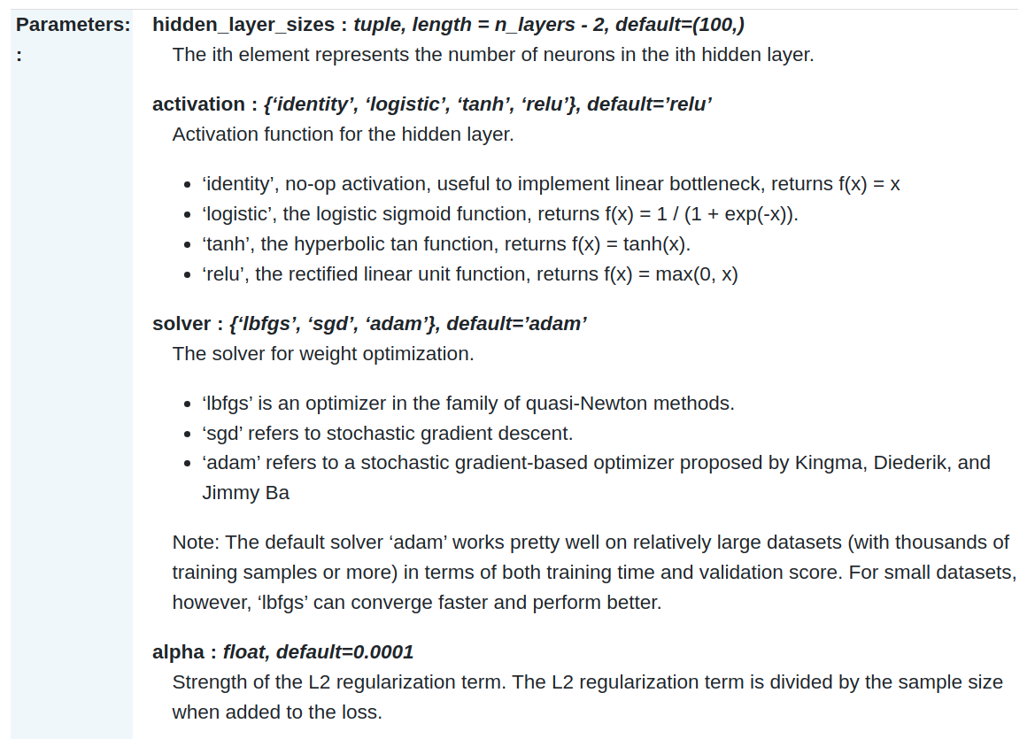- To limit the total execution time, you can do the following: - Use the algorithm name ``` AutoGluon_param_time_limit: 60*5 ``` - Explicitly specify the algorithm category ``` AutoGluonRegressor_param_time_limit: 60*5 ``` - <span id="footnote_experimental_algorithm_name"></span>**Q & A**: - **How to set parameters for machine learning algorithms that are not in the above table?** To use a machine learning algorithm that is not in the above table, the user needs to explicitly specify the [**algorithm category**](#footnote_experimental_algorithm_class_list) provided by the `ml-sklearn` image. Using the algorithm category as a keyword, find the corresponding algorithm category in the official [**scikit-learn documentation**](https://scikit-learn.org/stable/modules/classes.html), and then click to find the parameters that can be used by the algorithm category.<br> For example, if you want to use `MLPRegressor`, you can find it by searching for keywords on this page, as follows:  Then click again, you can see the relevant parameter usage.  ### 4.3 Practical Examples The first example will be used to describe the actual operation process; the subsequent examples will be briefly explained. #### 4.3.1 If You Want to Spend More Time Finding the Optimal Algorithm And Hyperparameters, You Need to Increase the Calculation Time. This section is a supplementary note for when [**MODEL_ALGORITHM**](#MODEL_ALGORITHM) is set to the `Auto` option. In the [**parameter description**](https://automl.github.io/auto-sklearn/master/api.html) of **AutoRegressor**, it is mentioned: - **`time_left_for_this_task` (total time for the task)** > The preset time is 3600 seconds (1 hour) in seconds. > > The total time limit for searching for the best model. By increasing this value, AutoRegressor is more likely to find a better model. - **`per_run_time_limit` (time limit for a single execution)** > The preset time is 360 seconds (6 minutes) in seconds. > > Time limit for a single test with a selected model and a set of parameters. > > Some algorithms (such as MLP) may take longer to fit the model in a single test, and once the execution time exceeds the default 6 minutes, the algorithm is marked as a failure and is not included in the list of reference models. 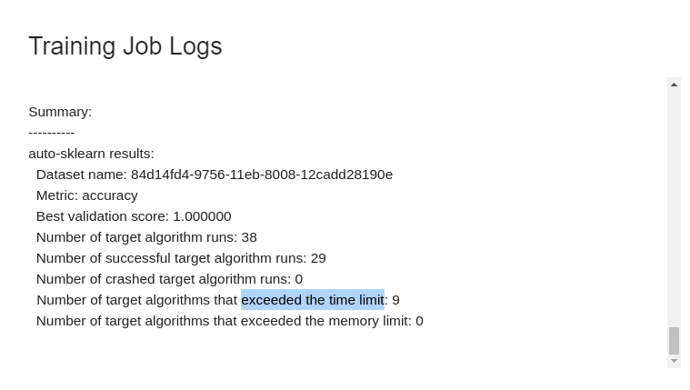When should this parameter be adjusted? > See [**2.3.2 Machine Learning Execution Logs**](#232-Machine-Learning-Execution-Logs) section to learn how to view logs. When the proportion of time-out algorithms is too high, we can consider relaxing the time limit for a single execution without considering time and money and other costs. >  To increase the calculation time, you can do the following: | Parameter | Settings Value | Description | | --- | ----- | --- | | `AutoRegressor_param_time_left_for_this_task` | `60*60*24` | in seconds.<br> The total time is set to 24 hours, or `86400`. | | `AutoRegressor_param_per_run_time_limit` | `60*30` | in seconds.<br> The single test time is set to 30 minutes, or `1800`. 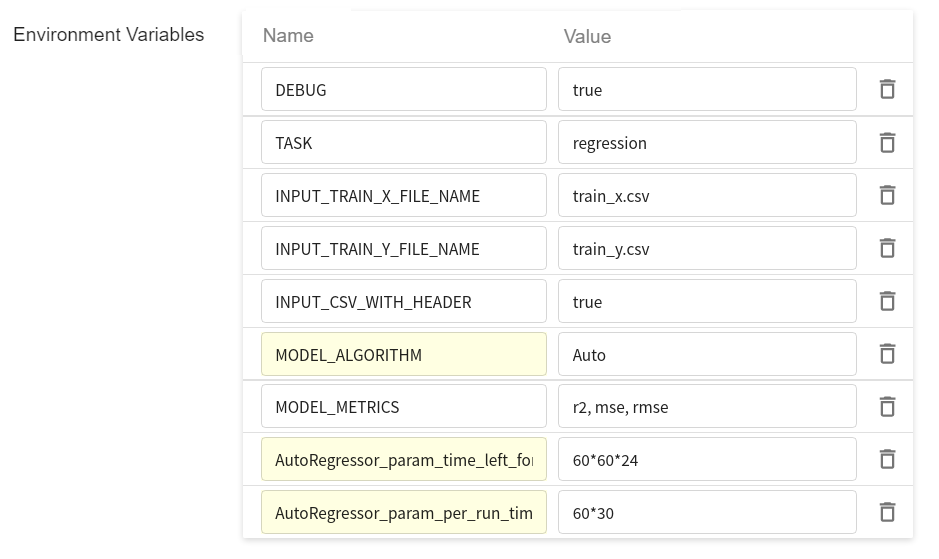| In the **Environment Variables** table of the [**Variable Settings**](#214-variable-settings) stage, actually enter two key values:  Training jobs that are started subsequently will use this setting. :::info :bulb: **Tips: More Settings and Configurations** In the section 2.1.2 [**Hardware Settings**](#212-Hardware-Settings), there are references to hardware resources for your own needs. To make use of the allocated hardware resources, you can do the following: | Parameter | Settings Value | Description | | --- | ----- | --- | | `AutoRegressor_param_n_jobs` | `-1` | Use all CPUs. The original default is a single core. | | `AutoRegressor_param_memory_limit` |`1024*40` |Increase the memory limit to 40GB to handle millions of table data.| ::: :::warning :warning: **Note:** The setting of algorithm parameters must be used together with the **`MODEL_ALGORITHM`** parameter; otherwise, the setting of algorithm parameters will be ignored. ::: #### 4.3.2 The Number of Iterations Is Not Enough, the Model Cannot Be Fit And Finalized, And the Number of Iterations Needs to Be Increased. | Parameter | Settings Value | Description | | --- | ----- | --- | | `SGDRegressor_param_max_iter` | `5000` | The default value of SGDRegressor is 1000. | #### 4.3.3 There Are Different Calculation Methods in A Single Algorithm, And You Want to Choose Different Calculation Methods to Fit the Data | SVR parameter | Settings Value | Description | | ------- | ----- | --- | | `SVR_param_kernel` | `linear` | Set the kernel of SVR (SVM) to `linear` | | `SVR_param_kernel` | `poly` | Set the kernel of SVR (SVM) to `poly` | | `SVR_param_kernel` | `sigmoid` | Set the kernel of SVR (SVM) to `sigmoid` | #### 4.3.4 To Use A Polynomial-based Algorithm Which Can Increase the Complexity of the Model by Changing the Power (Exponential Part). For SVR settings, the following 3 settings are grouped together and need to be used together: | SVR parameter | Settings Value | Description | | ------- | ----- | --- | | `MODEL_ALGORITHM` | `SVM` | Using SVM algorithm | | `SVR_param_kernel` | `poly` | Set the kernel of SVR (SVM) to `poly` | | `SVR_param_degree` | `5` | Change the power of [polynomial](https://zh.wikipedia.org/wiki/%E5%A4%9A%E9%A0%85%E5%BC%8F) from default of 3 to 5 | #### 4.3.5 Change the Penalty Level (Penalty Points) Penalty is also known as regularization term, the generally available selections are L1, L2, and ElasticNet. | Parameter | Settings Value | Description | | --- | ----- | --- | | `SGDRegressor_param_penalty` | `elasticnet` | | | `SVR_param_C` | `2` | Set the penalty coefficient from the default of `1` to `2`; the higher the value of `C`, the less tolerance for errors, but it may overfit. |