---
description: OneAI Documentation
tags: Case Study, YOLO, CVAT, EN, Deprecated
---
[OneAI Documentation](/s/user-guide-en)
# AI Maker Case Study - YOLOv4 Image Recognition Application
:::warning
:warning: **Note:** This document is no longer maintained due to system or service updates. For new versions of documents or similar use cases, please refer to [**AI Maker Case Study - YOLOv7 Image Recognition**](/s/casestudy-yolov7-en)。
:::
[TOC]
## 0. Deploy YOLOv4 Image Recognition Application
In this example, we will build a YOLO image recognition application from scratch using the **`yolov4`** template provided by AI Maker for YOLOv4 image recognition application. The system provides **`yolov4`** template with pre-defined environment variables, image, programs and other settings for each stage of the task, from training to inference, so that you can quickly develop your own YOLO network.
The main steps are as follows:
1. [**Prepare the Dataset**](#1-Prepare-the-Dataset)
At this stage, we need to prepare the image dataset for machine learning training and upload it to the specified location.
2. [**Data Annotation**](#2-Data-Annotation)
At this stage, we will annotate objects in the image, and these annotations will later be used to train the neural network.
3. [**Training YOLO Model**](#3-Training-YOLO-Model)
At this stage, we will configure the relevant training job to train and fit the neural network, and store the trained model.
4. [**Create Inference Service**](#4-Create-Inference-Service)
At this stage, we deploy the stored model and make inferences.
5. [**Perform Image Recognition**](#5-Perform-Image-Recognition)
At this stage, we will demonstrate how to send inference requests using the Python language in Jupyter Notebook.
After completing this example, you will have learned to:
1. Familiarize yourself with AI Maker functions and create jobs for each stage.
2. Use AI Maker's built-in templates to create related jobs.
3. Use the storage service and upload data.
4. Use the CVAT tool to annotate objects for data preprocessing.
5. Perform object recognition through Jupyter Notebook.
6. Use the CVAT assisted annotation function to save time in manual annotation.
## 1. Prepare the Dataset
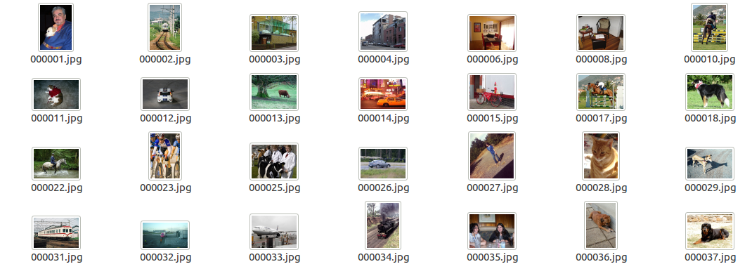
First, prepare the training datasets, such as: cats, dogs, flowers, etc. Follow the steps below to upload the dataset to the storage provided by the system, and store the dataset according to the specified directory structure for subsequent development.
### 1.1 Upload Your Own Dataset
If you have prepared your own dataset for training, please follow the steps below to store the data.
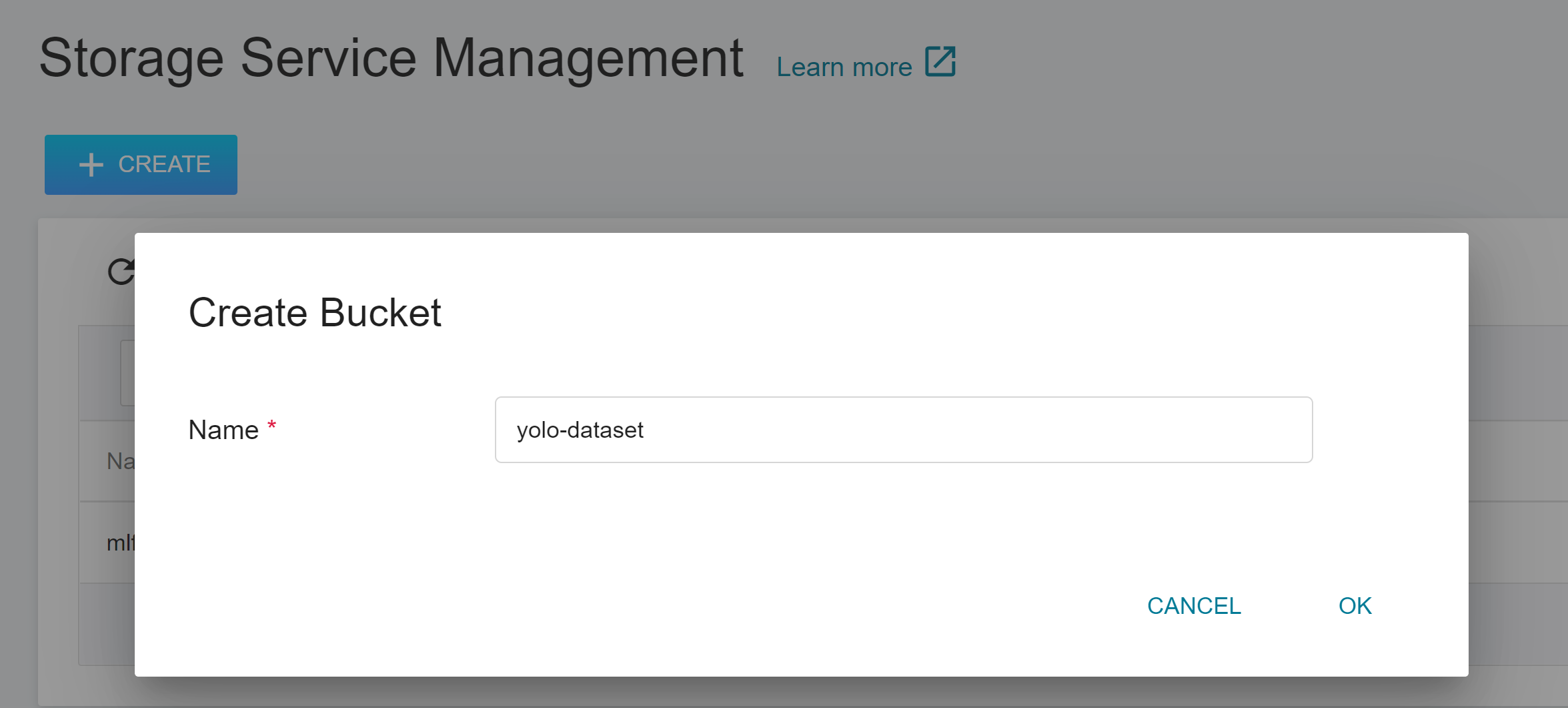
1. **Create a Bucket**
Select **Storage Service** from the OneAI service list menu to enter the Storage Service Management page, and then click **+CREATE** to add a bucket such as **yolo-dataset**. This bucket is used to store our dataset.
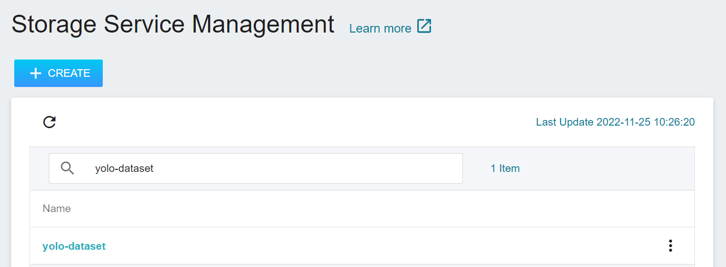
2. **View Bucket**
After the bucket is created, go back to the Storage Service Management page, and you will see that the bucket has been created.
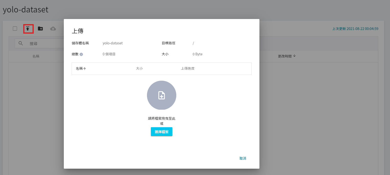
3. **Upload your own dataset**
Click the created bucket, and then click **UPLOAD** to start uploading the dataset. (See [**Storage Service**](/s/storage-en) Description).
### 1.2 Upload Your Own Dataset and Annotated Dataset
If you already have a dataset and annotated data, you can store your own data according to the tutorial in this section.
1. Create a bucket
Select **Storage Service** from the OneAI service list menu to enter the Storage Service Management page, and then click **+CREATE** to add a bucket such as **yolo-dataset**. This bucket is used to store our dataset.

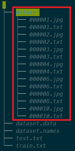
2. Add **dataset** folder
Please store the training images and the annotation text files in the dataset folder. The content of the text files is the data annotated with the annotation tool (for example: CVAT), for example:
```
3 0.716912 0.650000 0.069118 0.541176
```
Below are the descriptions from left to right:
```
3: Represents the class ID of the annotated object
0.716912: the ratio of the center coordinate X of the bounding box to the image width, which is the normalized center coordinate X of the bounding box.
0.650000: the ratio of the center coordinate Y of the bounding box to the image width, which is the normalized center coordinate Y of the bounding box.
0.069118: the ratio of the width of the bounding box to the width of the input image, which is the normalized width coordinate of the bounding box.
0.541176: the ratio of the height of the bounding box to the height of the input image, which is the normalized height coordinate of the bounding box.
```
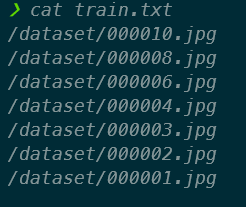
3. Add **train.txt** file
For 80% of all images in the file name list (or other ratios, can be changed on demand), YOLO will read the contents of the file in order to retrieve the photos for training, and the contents of the file will be linked to the image location with /dataset/.
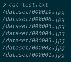
4. Add **test.txt** file
For 20% of all images in the file name list (or other ratios, can be changed on demand), YOLO will read the contents of the file in order to retrieve the photos for validation, and the contents of the file will be linked to the image location with /dataset/.
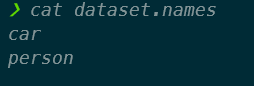
5. Add **dataset.names** file
The content of this file is a list of labels. YOLO needs to read this file during training and prediction. The labels in this example are car and person.
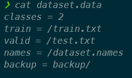
6. Add **dataset.data** file
Defines the number of labels and each configuration file, where backup is the location where the weight file (*.weights) is to be stored.
## 2. Annotation Data
In order for the YOLO network to learn and recognize the images we provide, we must first annotate the images to be trained. In this section, we will annotate the data to be trained by the **CVAT Tool (CVAT Computer Vision Annotation Tool)** integrated with **AI Maker**.
After the model is trained or if you already have a trained model, you can use the **CVAT Tool (CVAT Computer Vision Annotation Tool)** to reduce the time and cost of manual annotation, See [**6. CVAT Assisted Annotation**](#6-CVAT-assisted-annotation) in this tutorial.
:::info
:bulb: **Tips**: If you already have your own dataset and annotation data, you can go directly to step [**3. Training YOLO Model**](#3-Training-YOLO-Model).
:::
### 2.1 Enabling And Setting CVAT
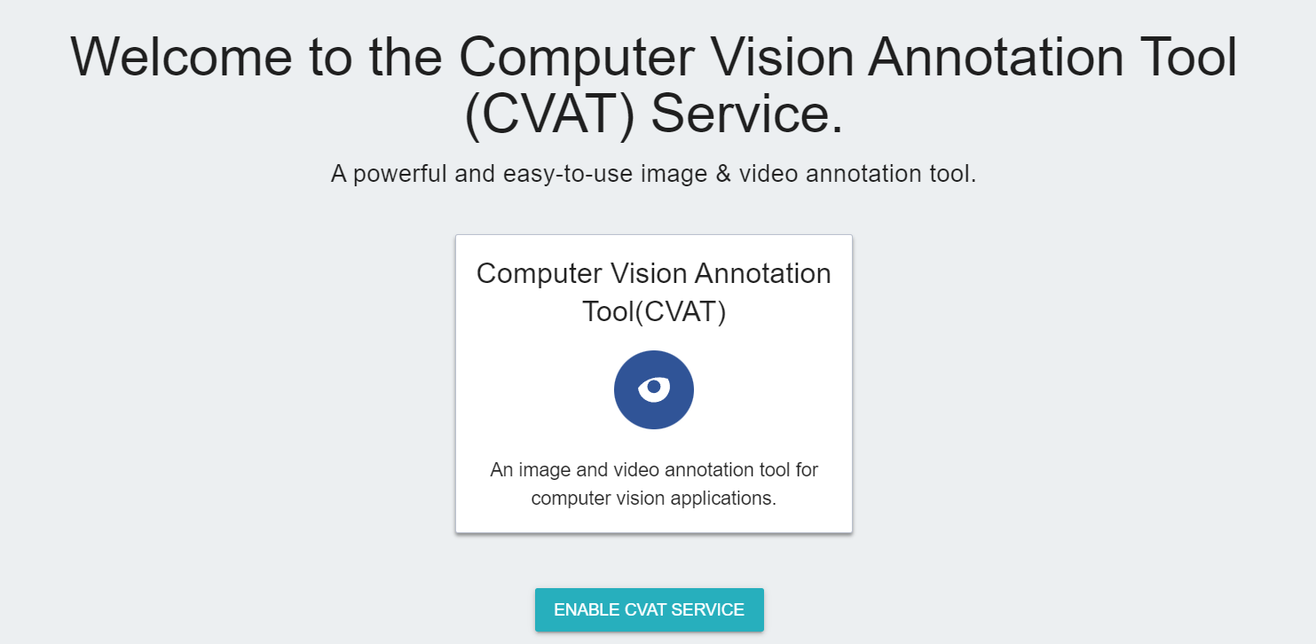
Click **Annotation Tools** on the left menu bar to enter the CVAT service home page. You need to click **Enable CVAT Service** if you are using it for the first time. Only one CVAT service can be enabled for each project.
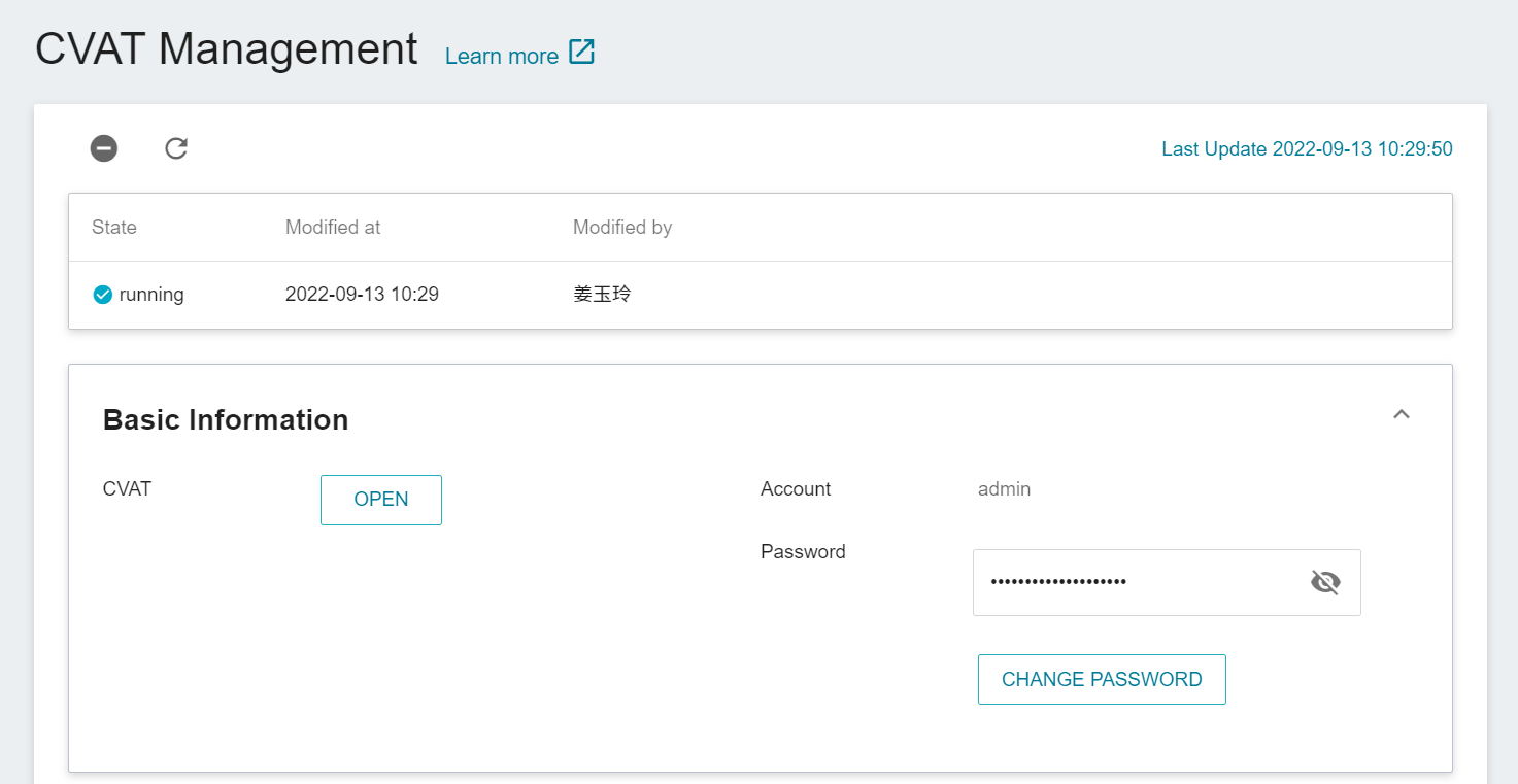
After CVAT is successfully enabled, the CVAT service link and account password will appear, and the status will be **`running`**. Click **OPEN** in the basic information to open the login page of the CVAT service in the browser.
:::info
:bulb: **Tips:** When CVAT is enabled for the first time, it is recommended to change the default password. This password has no expiration date and can be used by members of the same project to log in to CVAT service. For security reasons, please change the password regularly.
:::
### 2.2 Use CVAT to Create Annotation Task
1. **Login to CVAT**
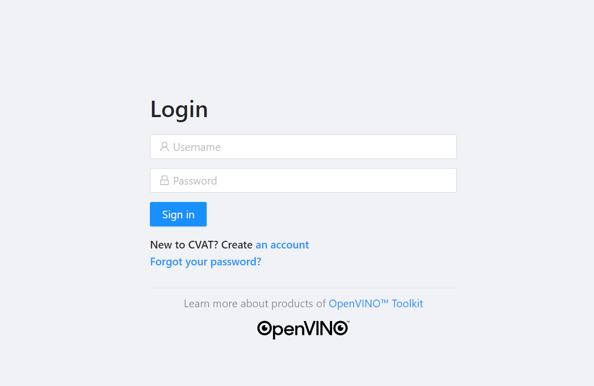
After clicking **Enable**, enter the account number and password on the **CVAT Service** login page to log in to the CVAT service.
:::warning
:warning: **Note:** Please use the Google Chrome browser to log in to CVAT. Using other browsers may cause unpredictable problems, such as being unable to log in or unable to annotate successfully.
:::
2. **Create CVAT Annotation Task**
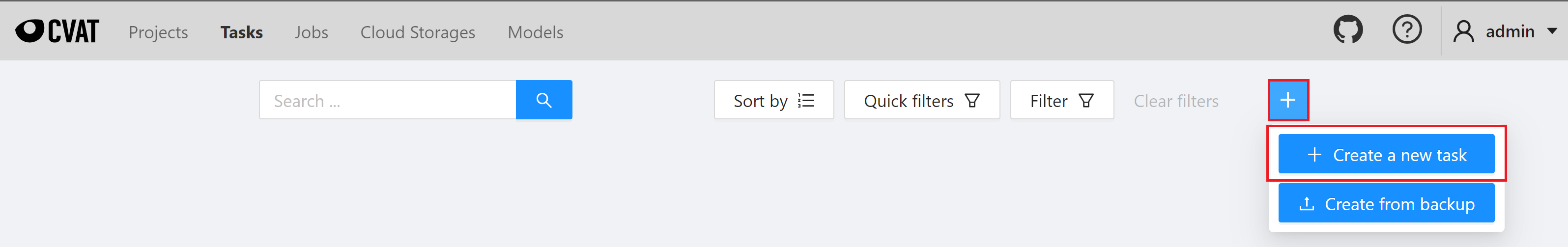
After successfully logging in to the CVAT service, click **Tasks** above to enter the Tasks page. Next click **+** and then click **+ Create a new task** to create an annotation task.
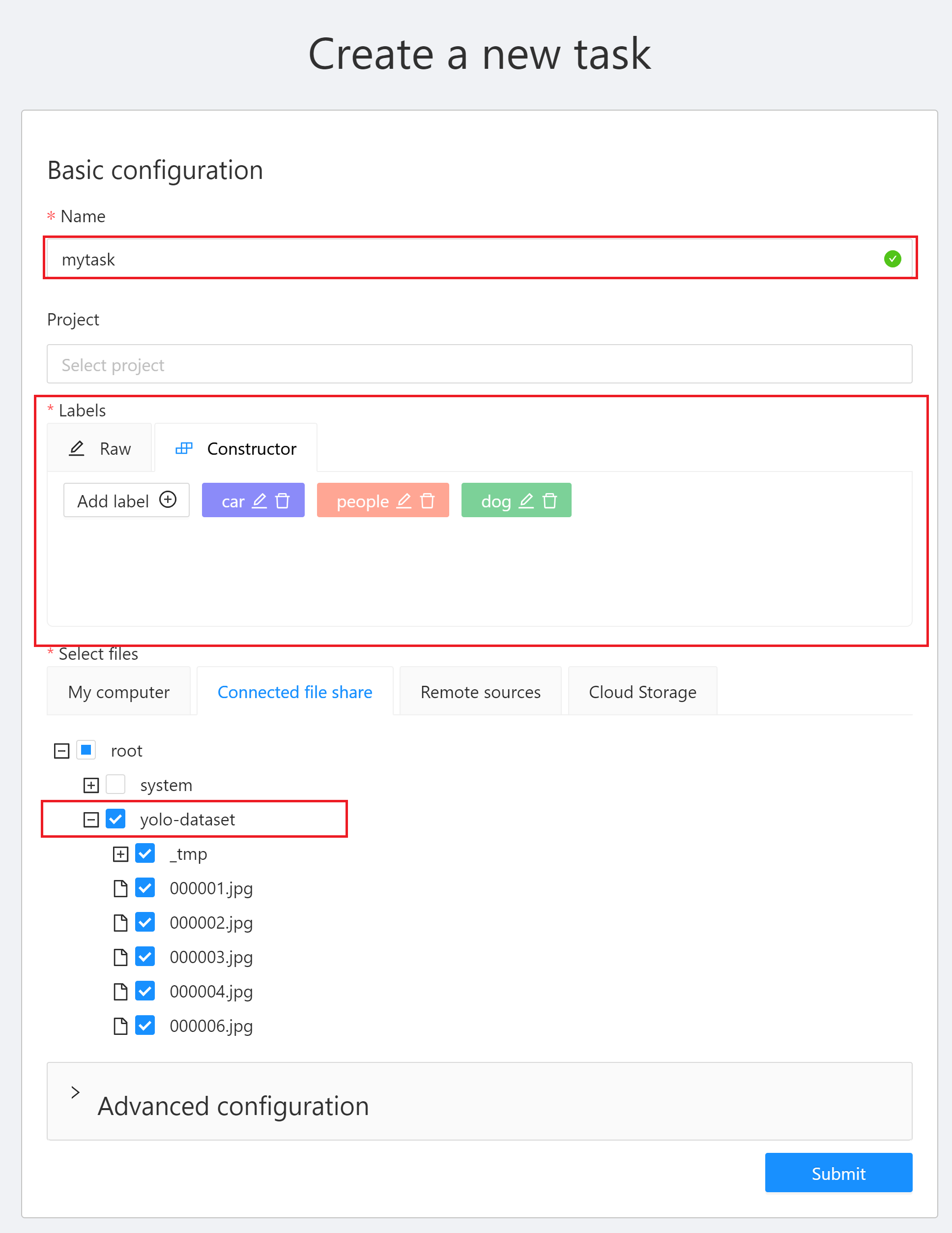
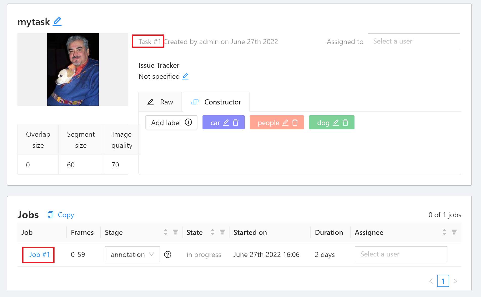
3. There are three places in the **Create a new task** window that need to be set:
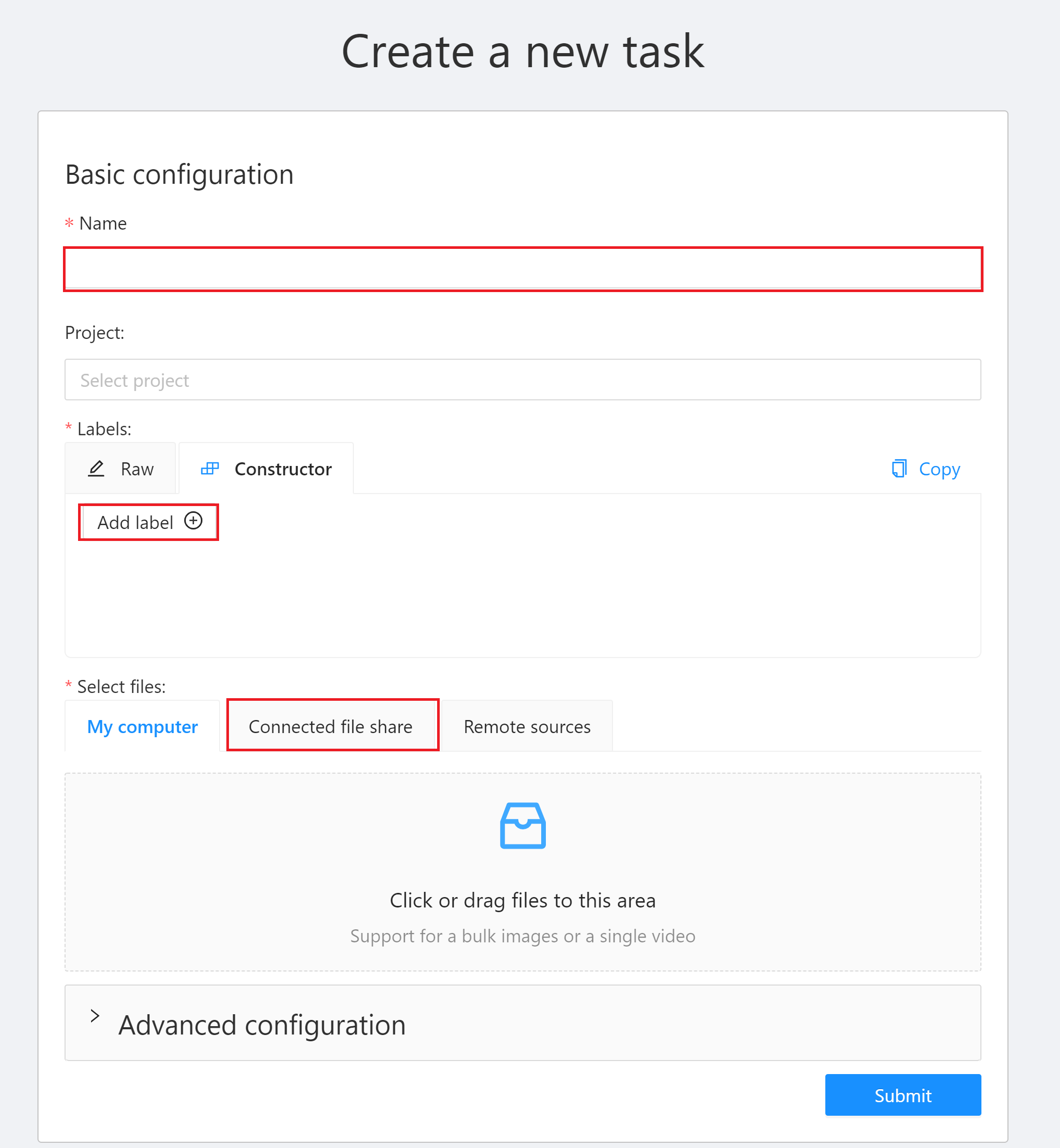
* **Name**: Enter a name for this Task, for example: `mytask`.
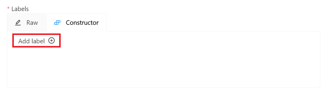
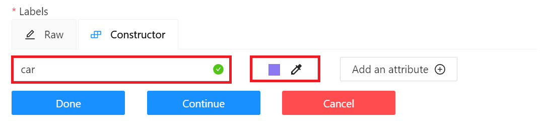
* **Labels**: Set the label of the object to be recognized. Click **Add label**, enter the label name, click the color block on the right to set the color of the label, then click **Continue** to continue adding other labels, or click **Done** to complete the label setting. In this example, we will create three labels: car, people and dog.
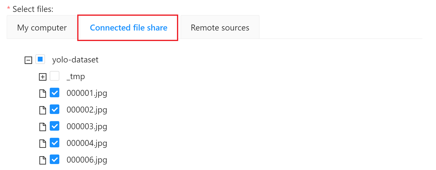
* **Select files**: Select the training dataset source. For this example, click **Connected file share** and select **`yolo-dataset`** bucket as the dataset source. For the dataset, please refer to [**1. Prepare the Dataset**](#1-prepare-the-dataset). After completing the setting, click **Submit** to create the Task.
:::warning
:warning: **Note: CVAT file size limit**
In the CVAT service, it is recommended that you use the bucket of the storage service as data source. If the data is uploaded locally, the CVAT service limits the file size of each TASK to 1 GB.
:::
### 2.3. Use CVAT for Data Annotation
After creating CVAT annotation task, you can then proceed to data annotation.
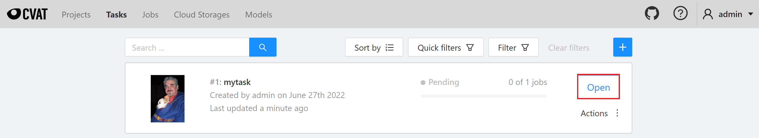
1. **View the Created Task**
After the annotation task is created, it will appear at the top of the **Tasks** list. Click **OPEN** to enter the task details page.
2. **Start Annotating**
On the task details page, the created object label will be displayed. After the label is confirmed, click **Job #id** to start annotating. Here, **`Task #1`** means that this Taskid is 1, and subsequent training tasks will need this information.
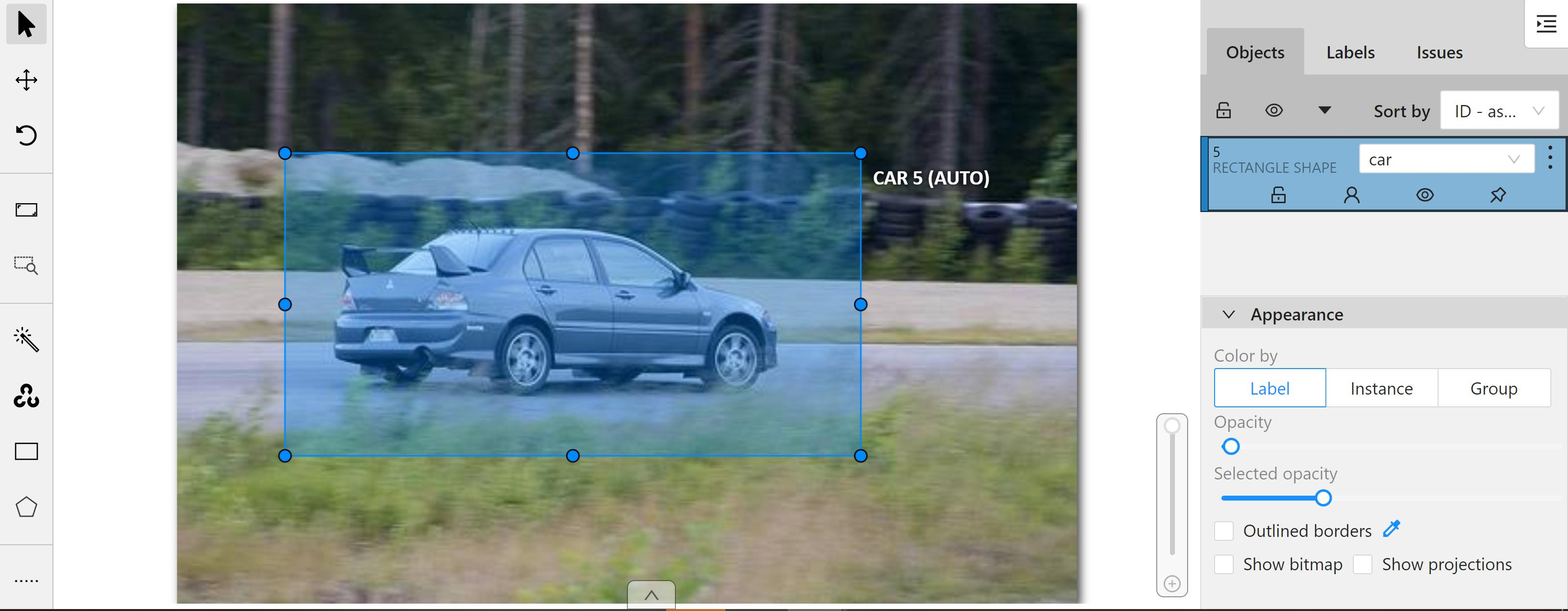
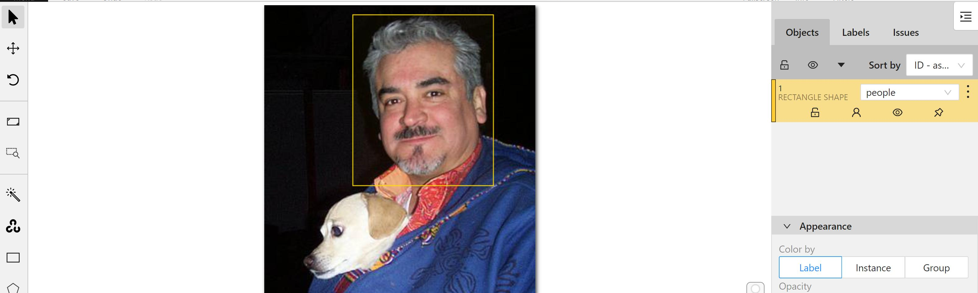
3. **Annotation**
You will see a picture you want to annotate after entering the annotation page. If there is a target object in the picture, you can annotate it according to the following steps.
1. Select the rectangle annotation tool **Draw new rectangle** on the left toolbar.
2. Select the label corresponding to the object.
3. Frame the target object.
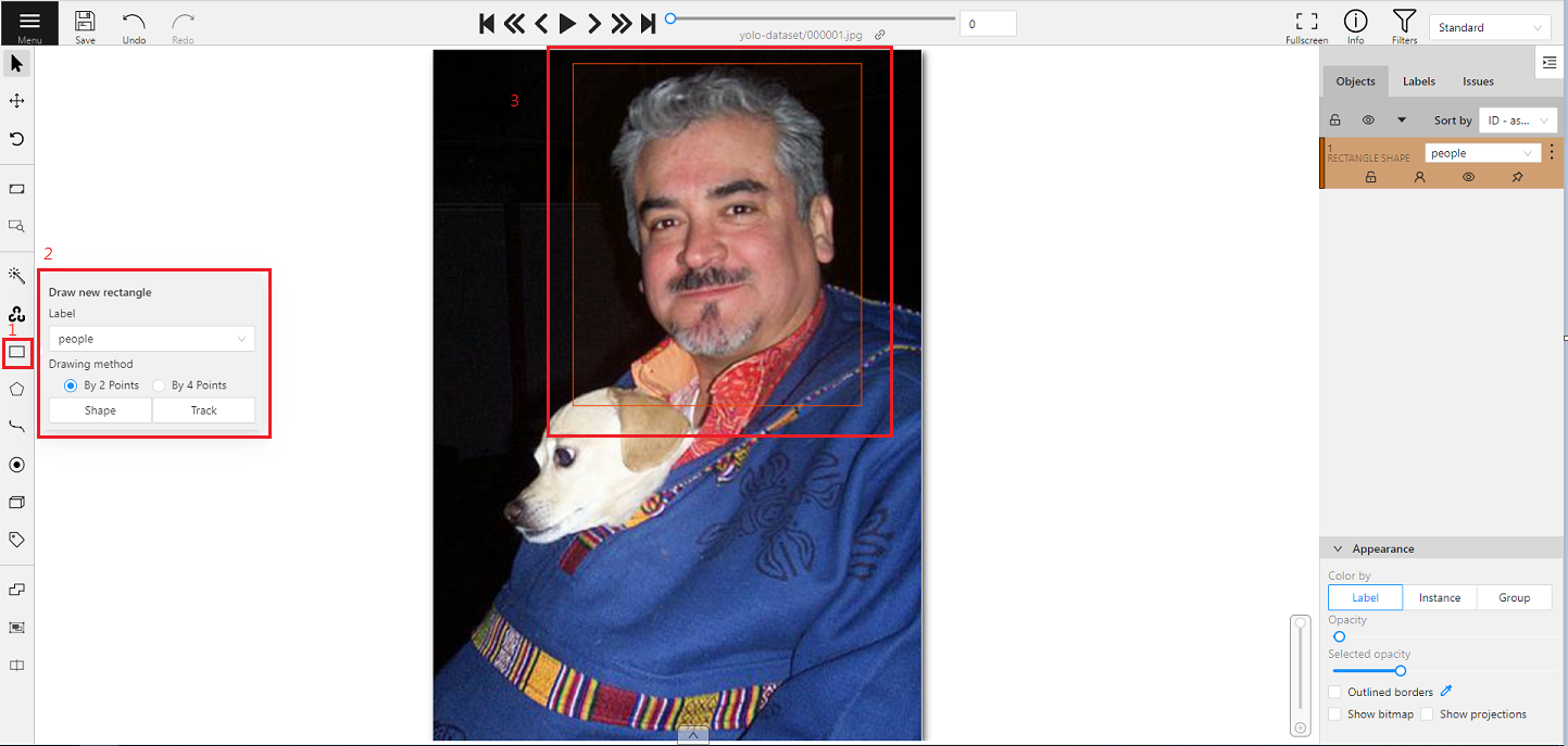
If there are multiple target objects in the picture, please repeat the annotating action until all target objects are annotated.
4. **Save Annotation Results**
After annotating several pictures, you can click **SAVE** in the upper left corner to save the annotation results, and continue with the subsequent tutorial.
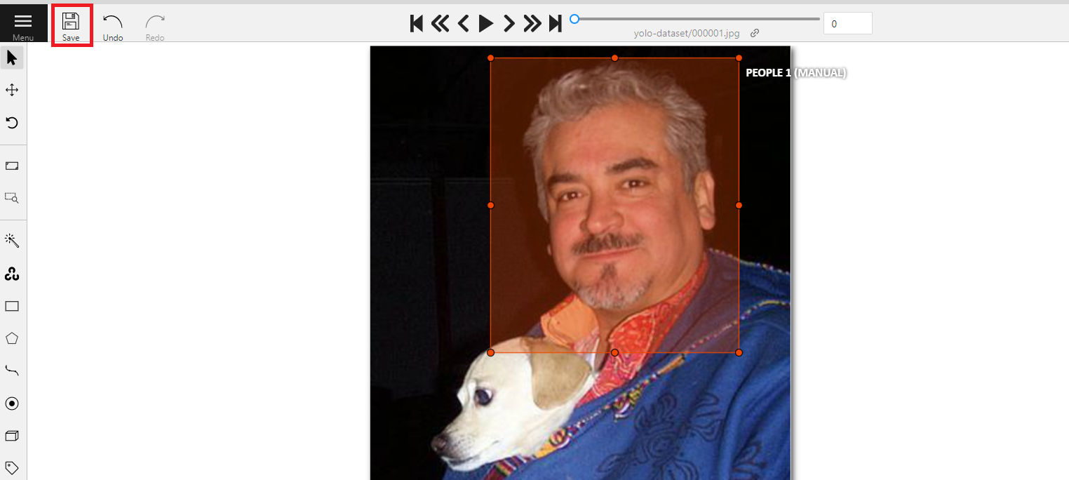
:::warning
:warning: **Note:** Make it a habit to save at any time during the annotation process, so as not to lose your work due to unavoidable incidents.
:::
### 2.4 Download Annotation Data
After the annotation is completed, the annotated data can be exported to the storage service, and then used in training model in AI Maker.
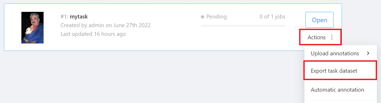
Go back to the **Tasks** page, click **Actions** on the right side of the task you want to download, and then click **Export task dataset**.
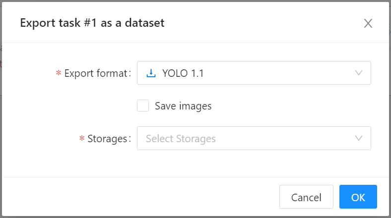
When the **Export task as a dataset** window appears, select the format of the annotation data to be exported and the bucket. This example will export the annotation data in **YOLO 1.1** format to the **`yolo-dataset`** bucket.
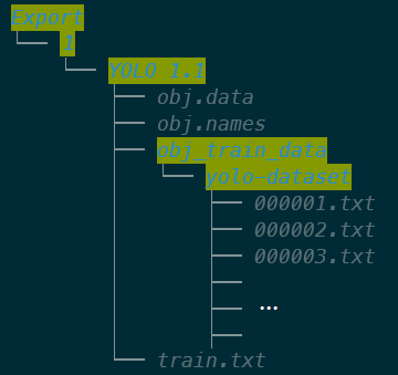
At this point, when you return to the bucket **`yolo-dataset`**, there will be an **Export** folder, and the downloaded annotation data will be stored according to the path of the Task id and data format. In this example, the Task id is 1 and the format is **YOLO 1.1**, so the downloaded annotation data will be placed in the **/Export/1/YOLO 1.1/** folder.
## 3. Training YOLO Model
After completing data [**Preparation**](#1-Prepare-the-Dataset) and [**Data Annotation**](#2-Annotation-Data), you can use these data to train and fit our YOLO network.
### 3.1 Create Training Jobs
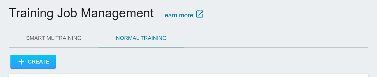
Select **AI Maker** from the OneAI service list, and then click **Training Jobs**. After entering the training job management page, switch to **Normal Training Jobs**, the click **+CREATE** to add a training job.
#### 3.1.1 Normal Training Jobs
There are five steps in creating a training job:
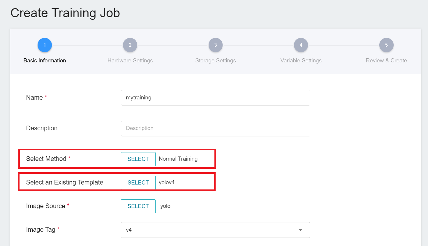
1. **Basic Information**
Let's start with the basic information setting. We first select **Normal Training Jobs** and use the built-in **`yolov4`** template to bring in the environment variables and settings. The setting screen is as follows:
2. **Hardware Settings**
Select the appropriate hardware resource from the list with reference to the current available quota and training program requirements.
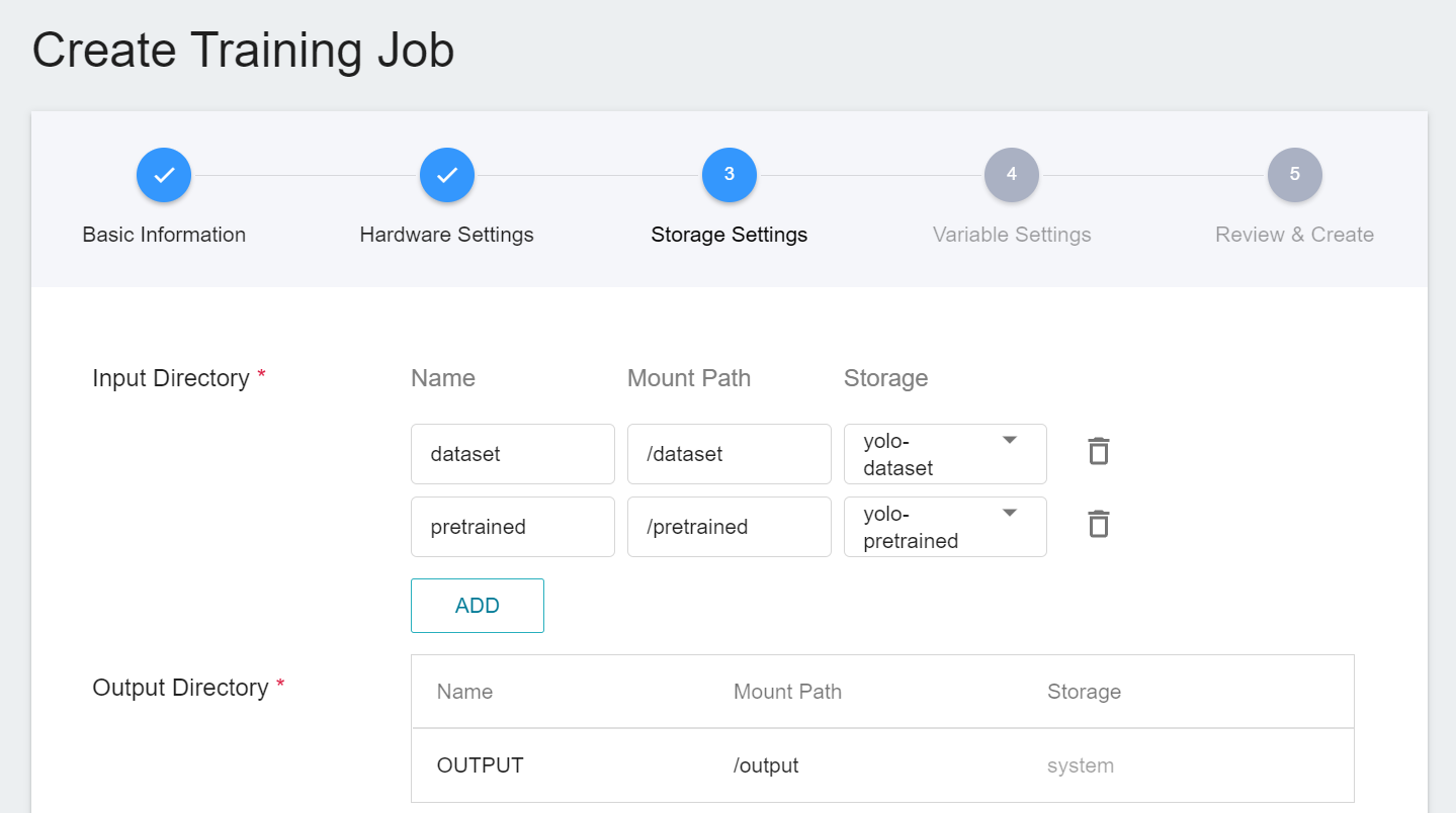
3. **Storage Settings**
There are two buckets to be mounted by default at this stage:
1. **dataset**: the bucket **`yolo-dateset`** where we store data.
2. **pretrained**: If you have a pretrained weight file to import, please name the pretrained weights file **`pretrained.weights`** and put it in the corresponding bucket, for example: **`yolo-pretrained`**, and then mount this bucket; if you have no pretrained weight, you can click the delete icon on the back to delete the mount path. AI Maker will use the built-in pretrained weight for training.
<br>
:::info
:bulb: **Tips: Pretrained weights built into the system**
To speed up training convergence, the system has a built-in pretrained weight file [**yolov4.weights**](https://github.com/AlexeyAB/darknet/releases/download/darknet_yolo_v3_optimal/yolov4.weights " https://github.com/AlexeyAB/darknet/releases/download/darknet_yolo_v3_optimal/yolov4.weights") trained by COCO datasets.
:::
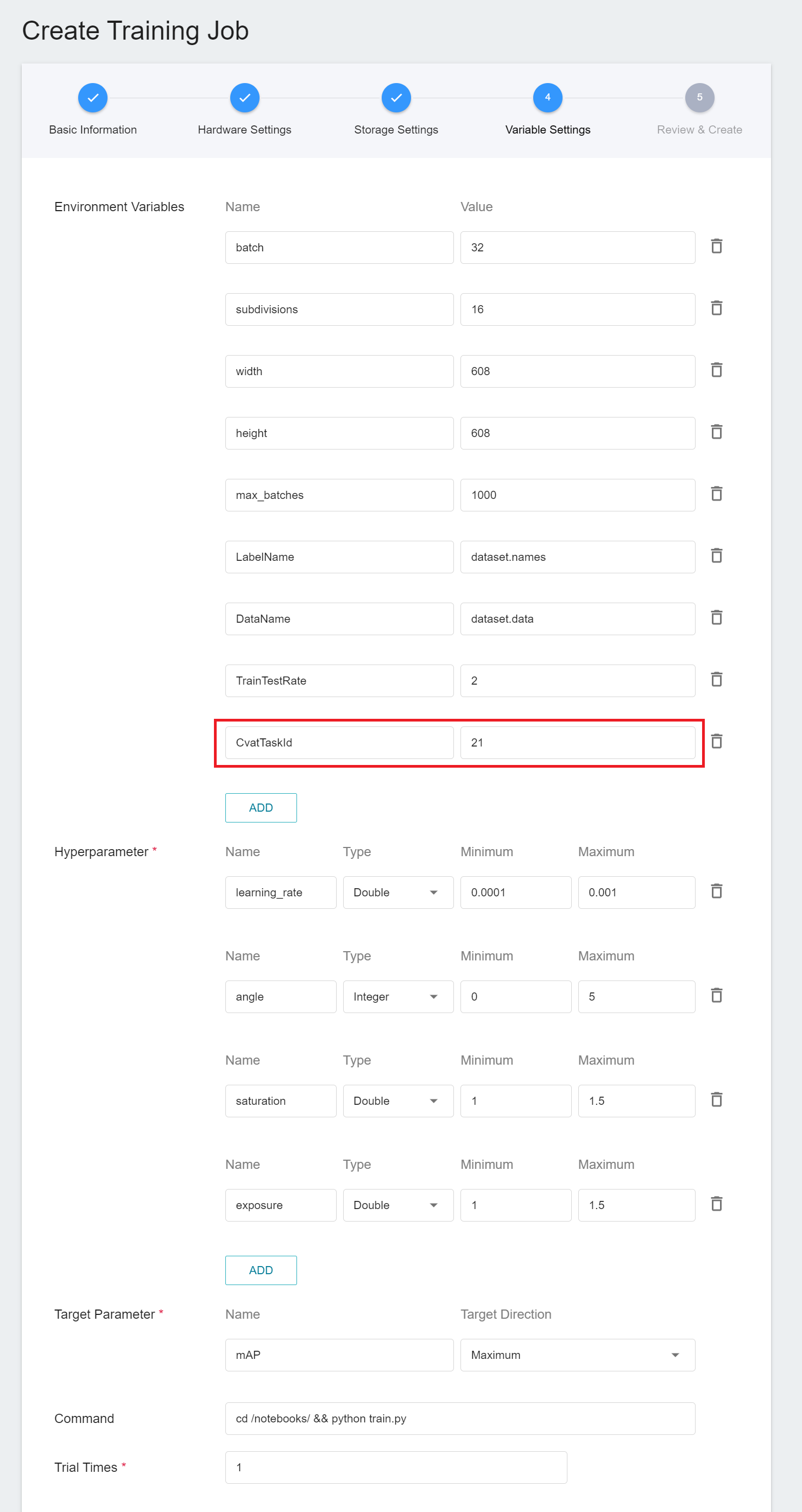
4. **Variable Settings**
The next step is to set environment variables and commands. The description of each field is as follows:
| Field name | Description |
| ----- | ----- |
| Environment Variables | Enter the name and value of the environment variables. The environment variables here include settings related to the training execution as well as the parameters required for the training network. |
| Target Parameter | After training, a value will be returned as the final result. Here, the name and target direction are set for the returned value. For example, if the returned value is the accuracy rate, you can name it accuracy and set its target direction to the maximum value; if the returned value is the error rate, you can name it error and set its direction to the minimum value. |
| Command | Enter the command or program name to be executed. For example: `python train.py`. |
However, because we have applied the **`yolov4`** template when filling in the basic information, the usual commands and parameters will be automatically imported. However, the value of CvatTaskId needs to be changed to the TaskId value of the downloaded annotation data in Step [**2.4 Downloading Annotation Data**](#24-Download-Annotation-Data).
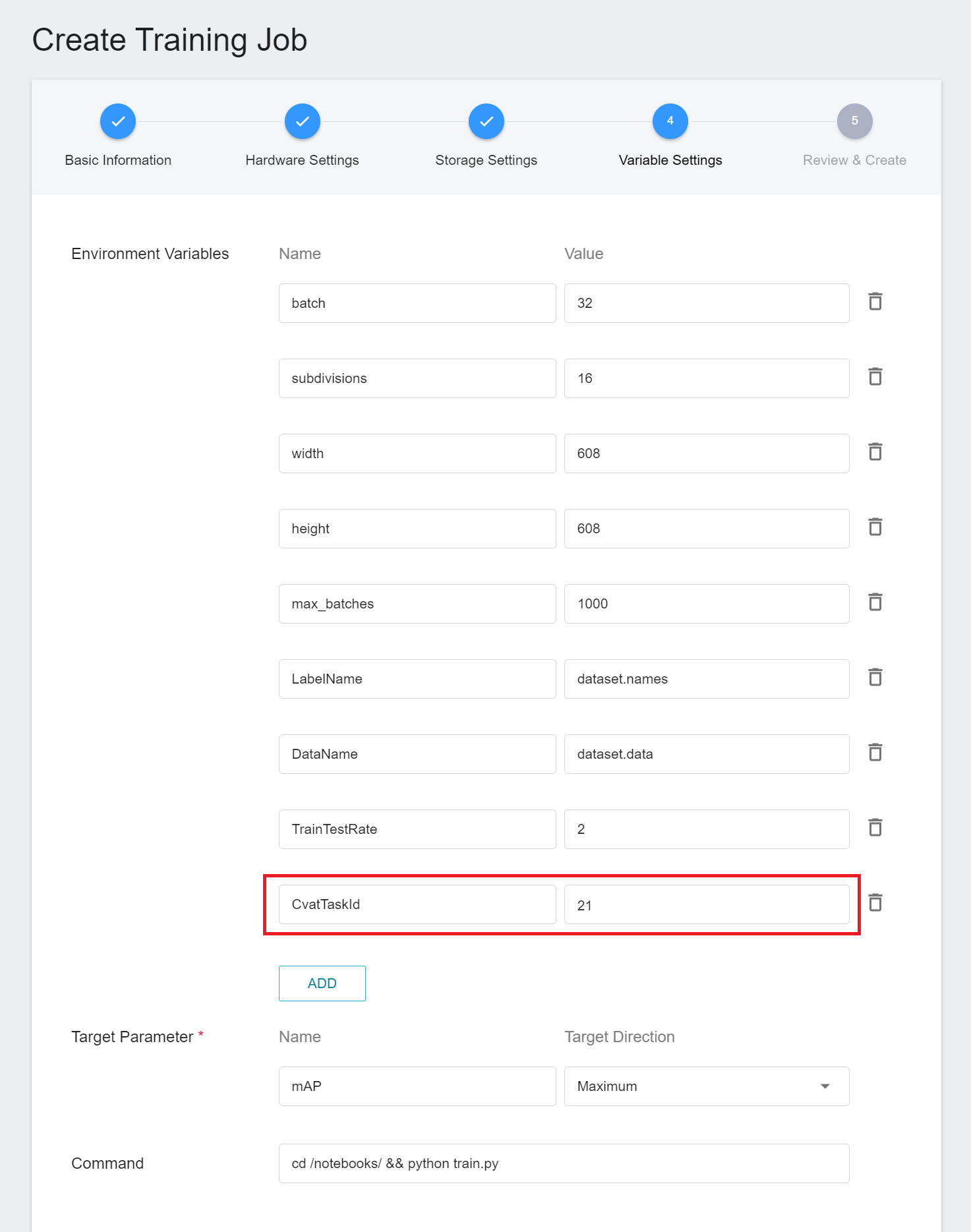
The setting values of environment variables can be adjusted according to your development needs. Here are the descriptions of each environment variable:
| Variable | Default | Description |
| ----- | -------| ---- |
|batch |32 |batch size, the size value of each batch, and the model is updated once per batch.|
| subdivisions |16 |Divide each batch into several parts to run according to the GPU memory. The larger the number of divided parts, the smaller the GPU memory required and the slower the training speed.|
|width |608 |Set the width of the picture to enter the network.|
|height |608 |Set the Height of the picture to enter the network.|
| max_batches | 1000 | The maximum number of batches to be run in this training. For the first training, it is recommended to run 1000 times for each additional category you want to identify.|
|LabelName |dataset.names | Defines the name of the profile; the content is a list of labels.|
|DataName | dataset.data | Defines the name of the profile; the contents are the number of labels and directory of each profile and weights.|
|TrainTestRate |2 |The ratio of training set to test set.<br> 2 means that one of every two images is used as the test set. |
|CvatTaskId |==CVATTASKID== |Please modify this parameter value to the **Task ID** of the data to be annotated with **CVAT**. The Task ID can be queried on the Tasks page of CVAT. If you use your own dataset and annotation data, please set to **none**.|
5. **Review & Create**
Finally, confirm the entered information and click CREATE.
#### 3.1.2 Smart ML Training Jobs
In the [**previous section 3.1.1**](#311-Normal-Training-Jobs), we introduced the creation of **Normal Training Jobs**, and here we introduce the creation of **Smart ML Training Jobs**. You can choose just one training method or compare the differences between the two. Both processes are roughly the same, but there are additional parameters to be set, and only the additional variables are described here.
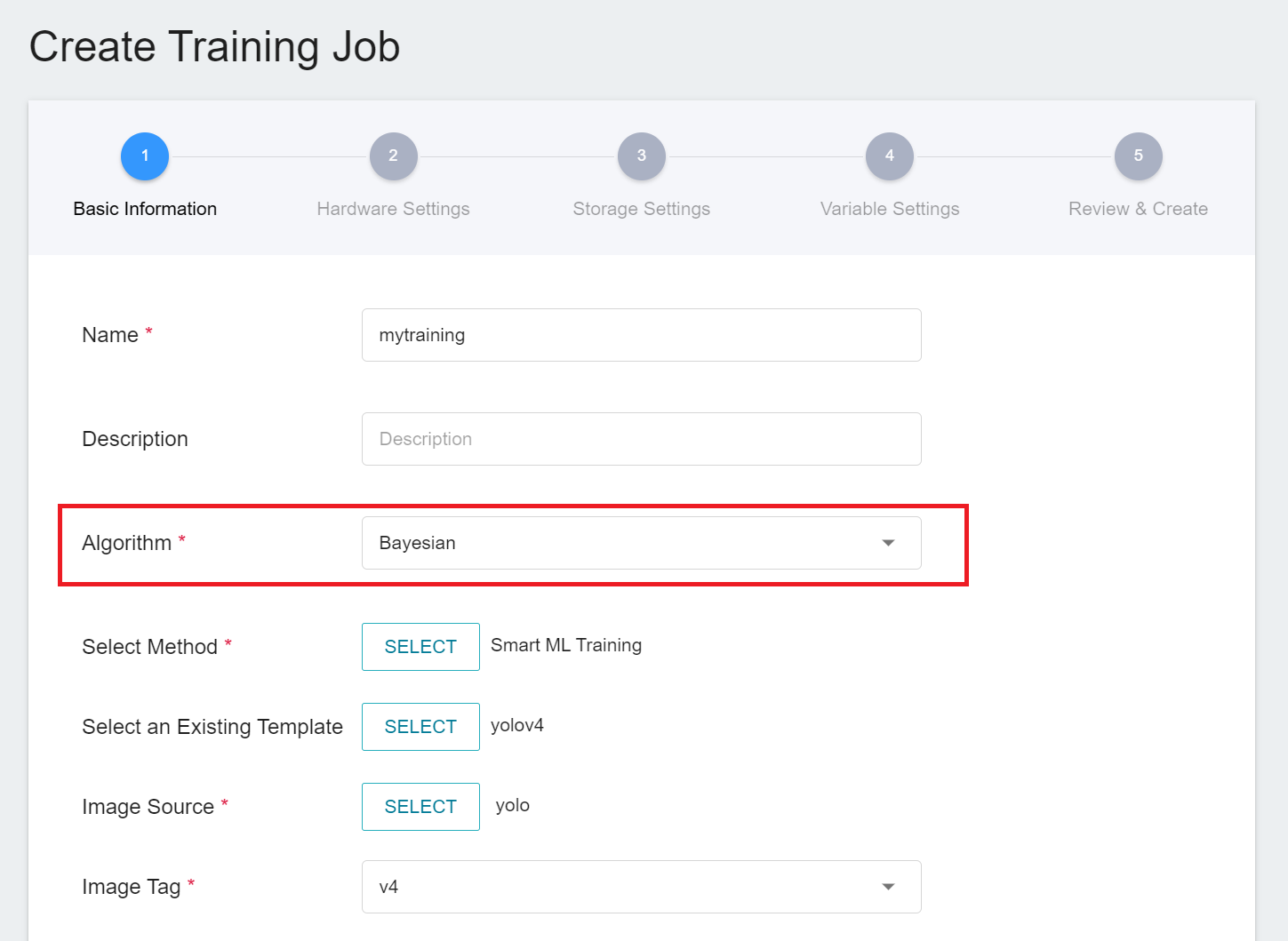
1. **Basic Information**
When Smart ML training job is the setting method, you will be further required to select the **Algorithm** to be used for the Smart ML training job, and the algorithms that can be selected are as follows.
- **Bayesian**: Efficiently perform multiple training jobs to find better parameter combinations, depending on environmental variables, the range of hyperparameter settings, and the number of training sessions.
- **TPE**: Tree-structured Parzen Estimator, similar to the Bayesian algorithm, can optimize the training jobs of high-dimensional hyperparameters.
- **Grid**: Experienced machine learning users can specify multiple values of hyperparameters, and the system will perform multiple training jobs based on the combination of the hyperparameter lists and obtain the calculated results.
- **Random**: Randomly select hyperparameters for the training job within the specified range.
2. **Variable Settings**
In the variable settings page, there will be additional settings for **Hyperparameter** and **Trial Times**:
- **Hyperparameter**
This tells the job what parameters to try. Each parameter must have a name, type, and value (or range of values) when it is set. After selecting the type (integer, float, and array), enter the corresponding value format when prompted.
| Name | Value range | Description |
| ---- | ---- | ---- |
| learning_rate | 0.0001 ~ 0.001 | The **Learning Rate** parameter can be set larger at the beginning of model learning to speed up the training. In the later stage of learning, it needs to be set smaller to avoid divergence. |
| angle | 0 ~ 5 | The **Angle** of the picture to be adjusted, setting it to 5 means the picture will be rotated by -5 ~ 5 degrees to get more samples.|
| saturation | 1 ~ 1.5 | The **Saturation** of the picture to be adjusted, setting it to 1.5 means that the saturation can be adjusted from 1 to 1.5 to get more samples.|
| exposure | 1 ~ 1.5 | The **Exposure** of the picture to be adjusted, setting it to 1.5 means that the exposure can be adjusted from 1 to 1.5 to get more samples. |
Of course, some of the training parameters in **Hyperparameter** can be moved to **Environmental Variables** and vice versa. If you want to fix a parameter, you can remove it from the **Hyperparameter** setting and add it to the **Environment Variable** with a fixed value; conversely, if you want to add the parameter to the trial, remove it from the environment variable and add it to the hyperparameter settings below.
- **Trial Times**
Set the number of training sessions, and the training job is executed multiple times to find a better parameter combination.
### 3.2 Start a Training Job
After completing the setting of the training job, go back to the training job management page, and you can see the job you just created.
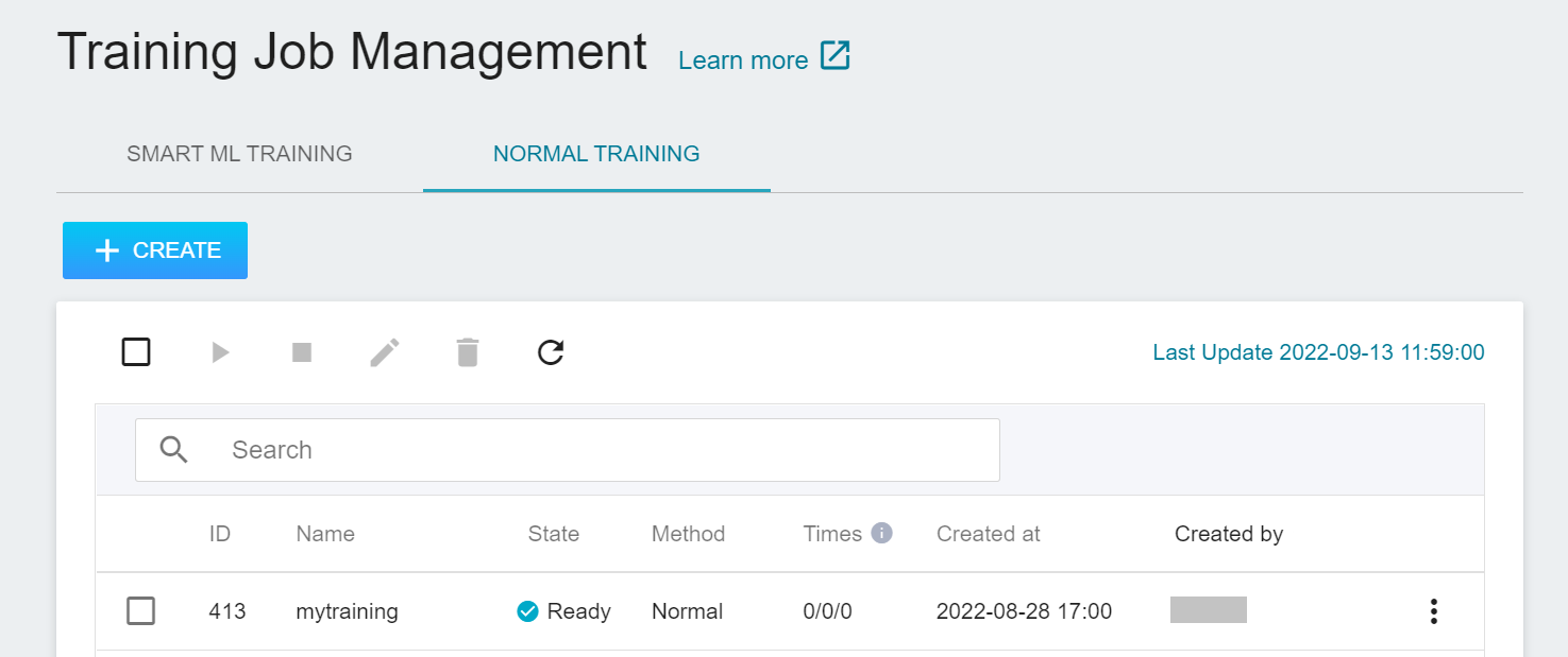
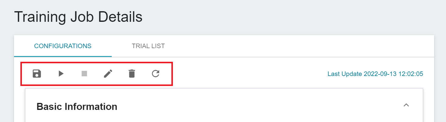
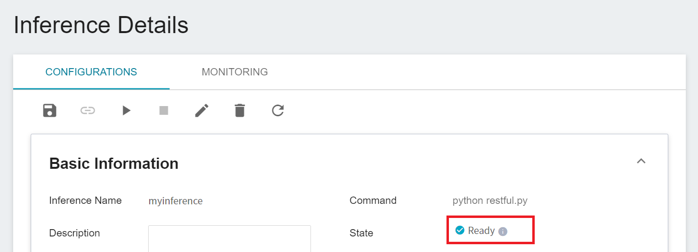
Click the job to view the detailed settings of the training job. The command bar has 6 icons: **Save (save as template)**, **START**, **STOP**, **EDIT**, **DELETE** and **REFRESH**. If the job state is displayed as **`Ready`** at this time, you can click **START** execute the training job.
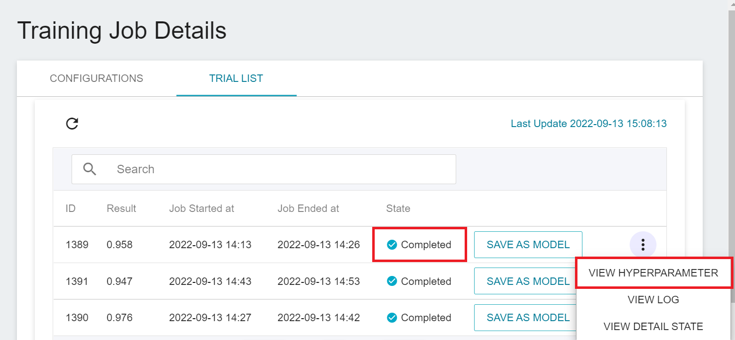
Once started, click the **Trial List** tab above to view the execution status and schedule of the job in the list. During training, you can click **VIEW LOG** or **VIEW DETAIL STATE** in the list on the right of the job to know the details of the current job execution.
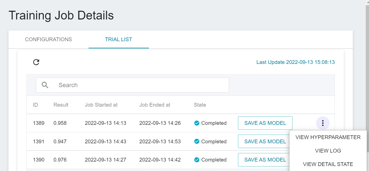
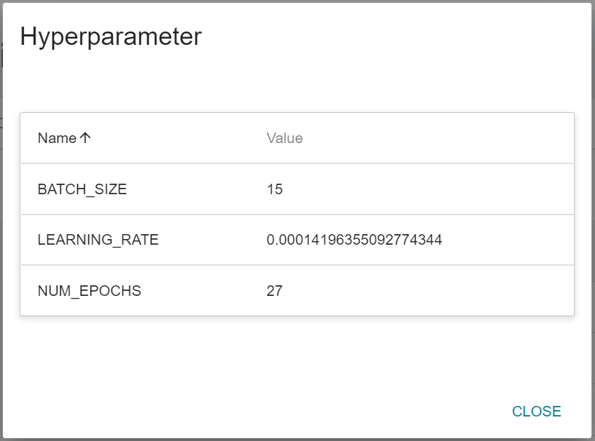
If you are running a Smart ML training job, a **View Hyperparameters** option will be added to the list, this option allows you to view the combination of parameters used for this training job.
### 3.3 View Training Results And Save Model
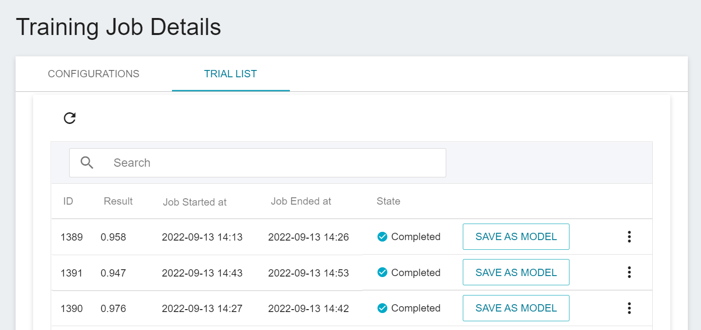
After the training job is completed, the job state in the Trial List page will change to **`Completed`** and the result will be displayed.
:::info
:bulb: **Tips: Send the results back to AI Maker**
The training results can be sent back to AI Maker through the functions provided by AI Maker. The training program used in this tutorial example already includes this program. If you use your own program, please refer to the following example:
* **ai.sendUpdateRequest({result})**: Return the training result (single value), such as error_rate or accuracy, the type must be int or float (int of Numpy type, float is not acceptable).
Below is an example:
```=
import AIMaker as ai
// your code
ai.sendUpdateRequest({result})
```
:::
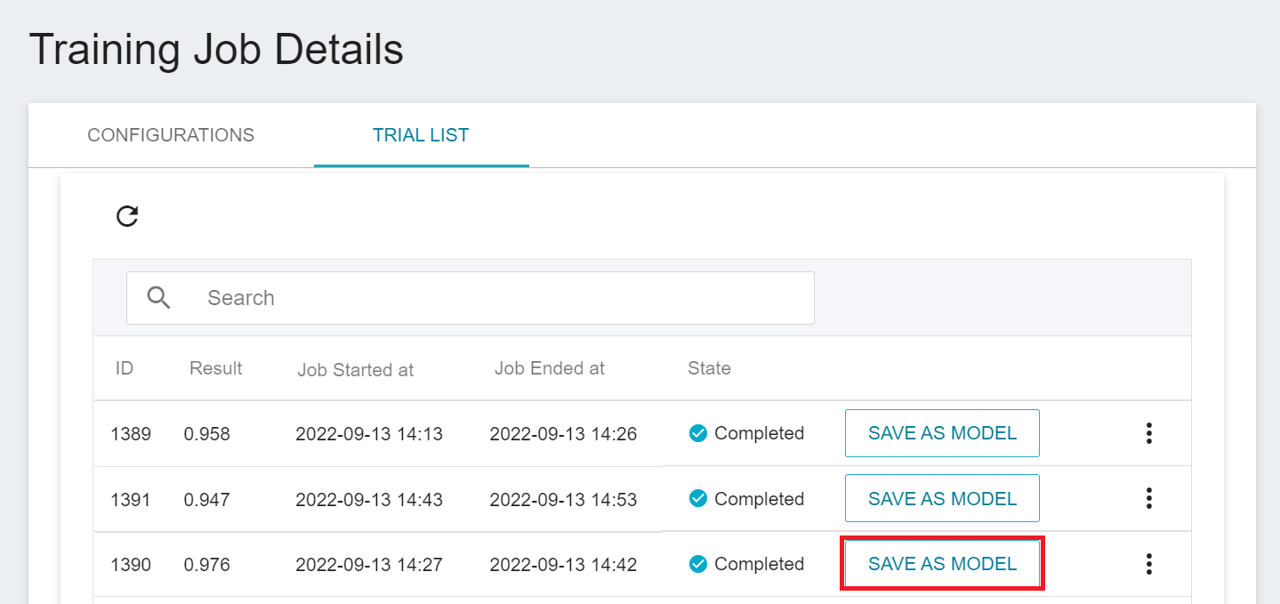
Observe the scores in the list, pick out the expected results, and store them in the model repository; if there are no expected results, readjust the values or value ranges of environmental variables and hyperparameters.
Below is a description of how to save the expected model to the model repository:
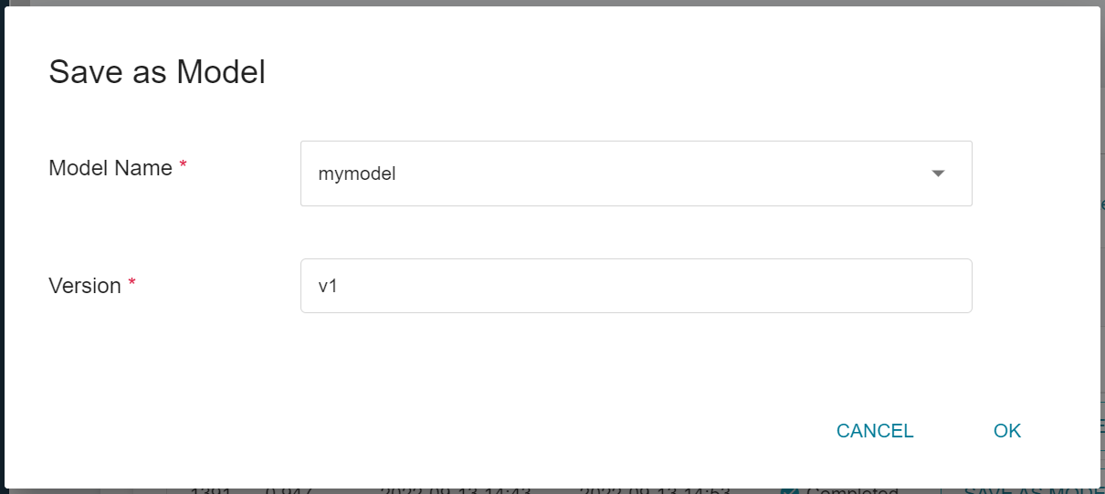
1. **Click Save as Model**
Click the **SAVE AS MODEL** button to the right of the training result you want to save.
2. **Enter the Model Name and Version Number**
A dialog box will appear, follow the instructions to enter the model name and version, and click OK when finished.
3. **View the Model**
Select **AI Maker** from the OneAI service list, and then click **MODEL**. After entering the model management page, you can find the model in the list.
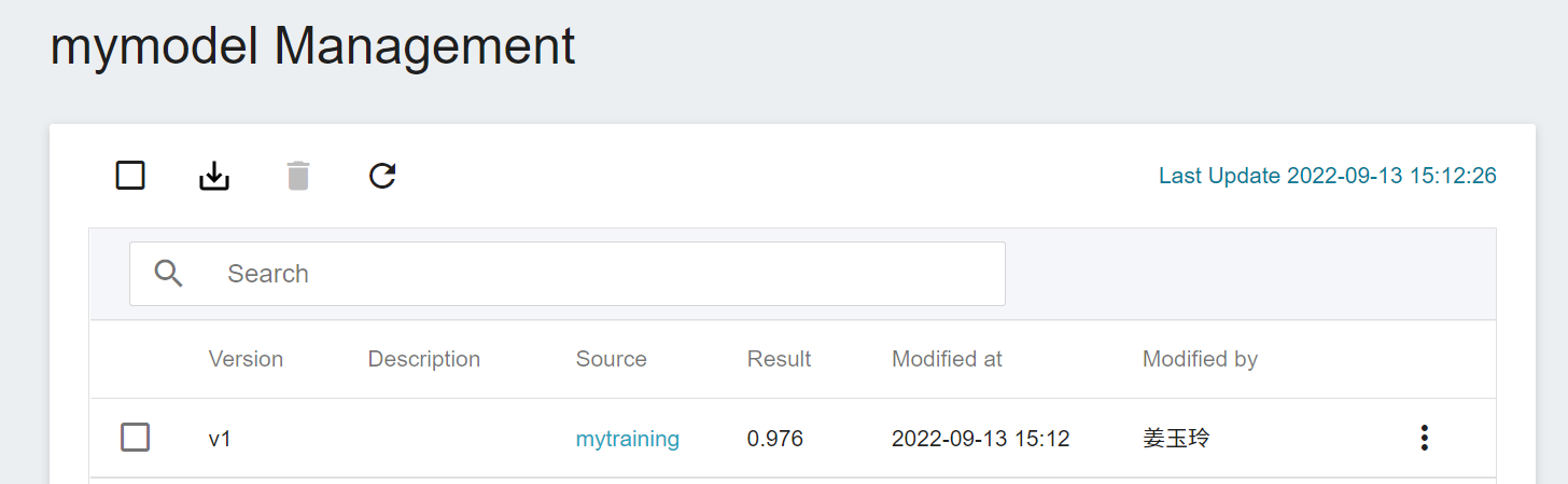
Click the model to enter the version list of the model, you can see all the versions, descriptions, sources, results and other information of the model.

## 4. Create Inference Service
After you have trained the YOLO network and stored the trained model, you can deploy it to an application or service to perform inference using the **Inference** function.
### 4.1 Create Inference
Select **AI Maker** from the OneAI service list, then click **Inference** to enter the inference management page, and click **+CREATE** to create an inference service. The steps for creating the inference service are described below:
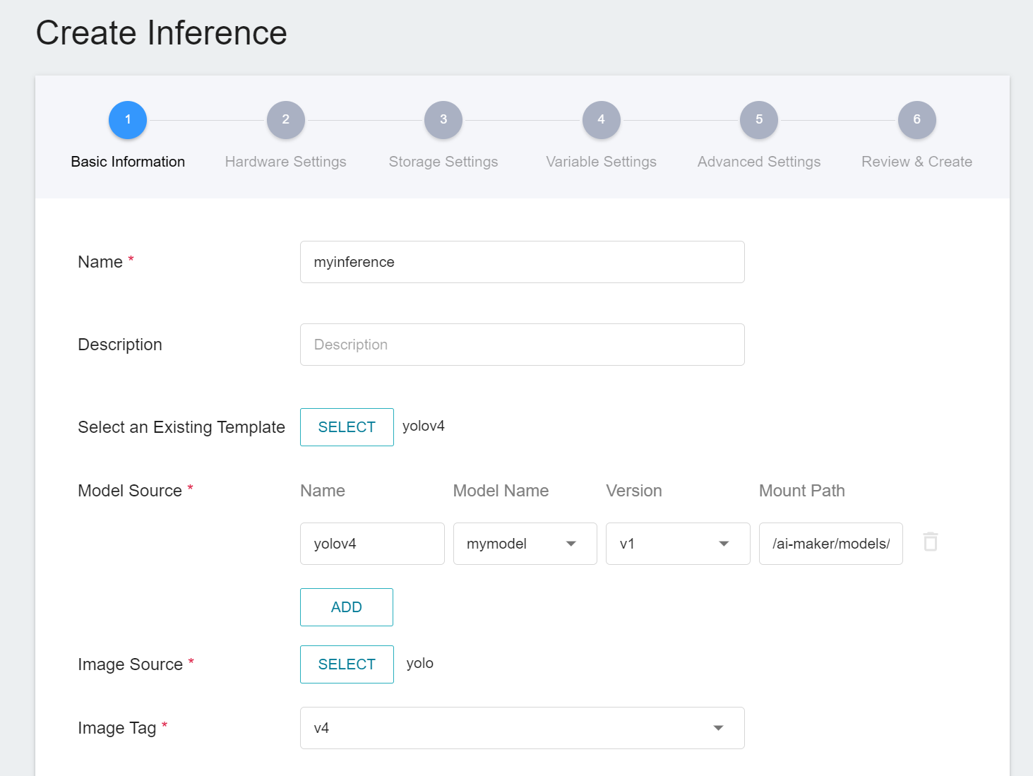
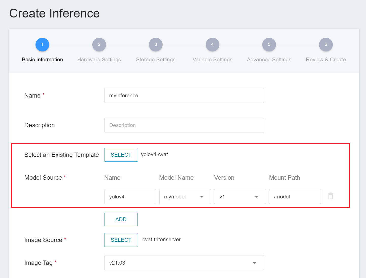
1. **Basic Information**
Similar to the setting of basic information for training jobs, we also use the **`yolov4`** inference template to facilitate quick setup for developers. However, the model name and version number to be loaded still need to be set manually:
- **Name**
The file name of the loaded model relative to the program's ongoing read, this value will be set by the `yolov4`inference template.
- **Model Name**
The name of the model to be loaded, that is, the model we saved in [**3.3 View training results and save model**](#33-view-training-results-and-save-model).
- **Version**
The version number of the model to be loaded is also the version number set in [**3.3 View training results and save model**](#33-view-training-results-and-save-model).
- **Mount Path**
Location of the loaded model relative to the program's ongoing read, this value will be set by the `yolov4` inference template.
2. **Hardware Settings**
Select the appropriate hardware resource from the list with reference to the current available quota and training program requirements.
3. **Storage Settings**
No configuration is required for this step.
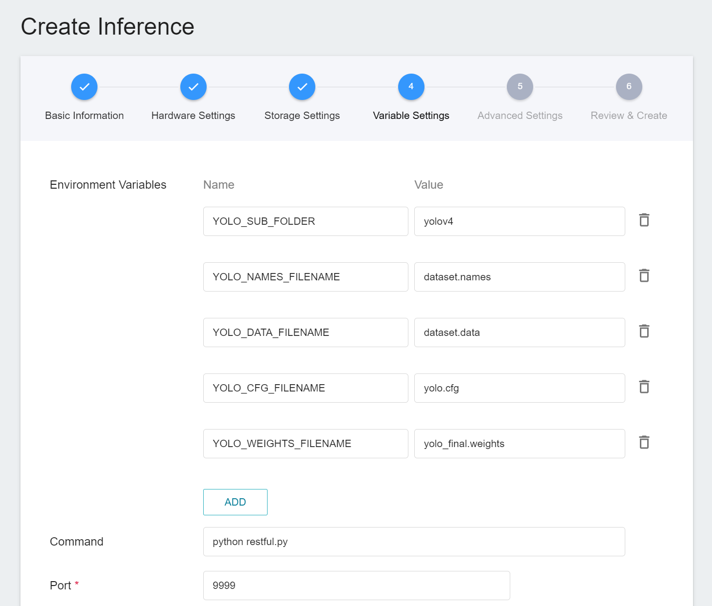
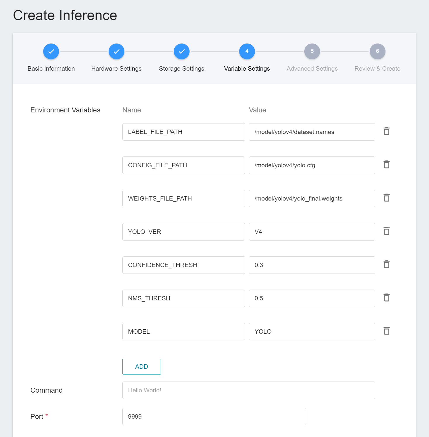
4. **Variable Settings**
In the Variable Settings page, these commands and parameters are automatically brought in when the **`yolov4`** template is applied.
5. **Advanced Settings**
* **Monitor Data**
The purpose of monitoring is to observe the number of API calls and inference statistics over a period of time for the inference service.
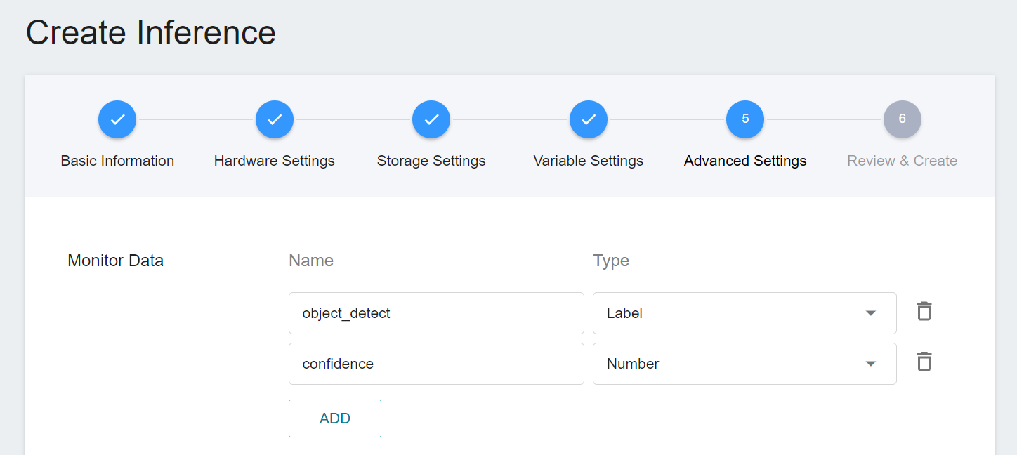
| Name | Type | Description |
|-----|-----|------------|
| object_detect | Tag | The total number of times the object has been detected in the specified time interval.<br> In other words, the distribution of the categories over a period of time.<br>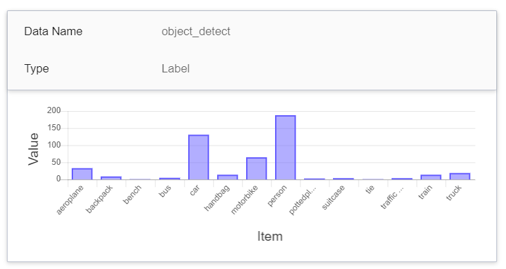|
| confidence | Number | The confidence value of the object being detected when the inference API is called once at a certain point in time.<br>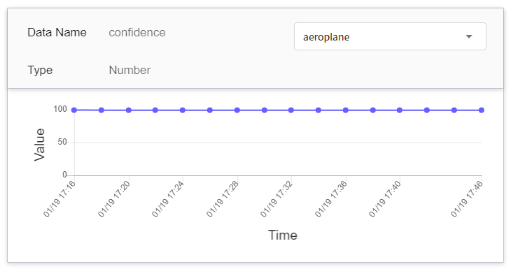
|
6. **Review & Create**
Finally, confirm the entered information and click CREATE.
### 4.2 Making Inference
After completing the settings of the inference service, go back to the inference management page, you can see the tasks you just created, and click the list to view the detailed settings of the service. When the service state shows as **`Ready`**, you can start connecting to the inference service for inference.
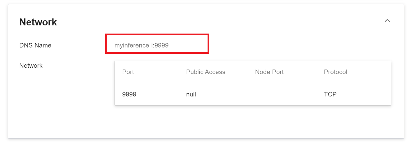
Worth noting is the **URL** in the detailed settings. Since the current inference service does not have a public service port for security reasons, we can communicate with the inference service we created through the **Container Service**. The way to communicate is through the **URL** provided by the inference service, which will be explained in the next section.
:::info
:bulb: **Tips:** The URLs in the document are for reference only, and the URLs you got may be different.
:::
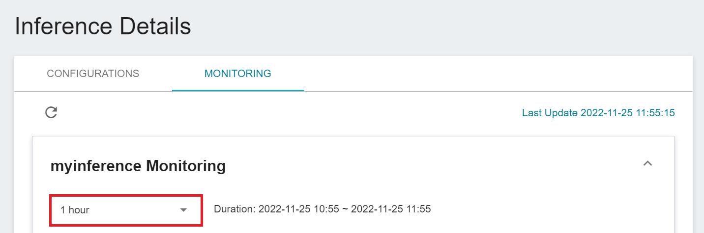
You can click on the **Monitor** tab to see the relevant monitoring information on the monitoring page, as shown in the figure below.
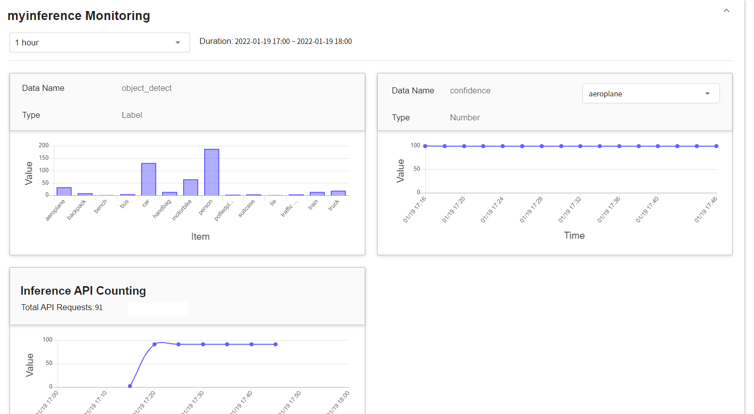
Click the Period menu to filter the statistics of the Inference API Call for a specific period, for example: 1 hour, 3 hours, 6 hours, 12 hours, 1 day, 7 days, 14 days, 1 month, 3 months, 6 months, 1 year, or custom.
:::info
:bulb: **Tips: About the start and end time of the observation period**
For example, if the current time is 15:10, then.
- **1 Hour** refers to 15:00 ~ 16:00 (not the past hour 14:10 ~ 15:10)
- **3 Hours** refers to 13:00 ~ 16:00
- **6 Hours** refers to 10:00 ~ 16:00
- And so on.
:::
## 5. Perform Image Recognition
In this section, we will explain how to use Jupyter Notebook to invoke the inference service.
### 5.1 Start Jupyter Notebook
This section describes how to use **Container Service** to start Jupyter Notebook.
#### 5.1.1 **Create Container Service**
Select **Container Service** from the OneAI service list. On the Container Service management page, click **+CREATE**.
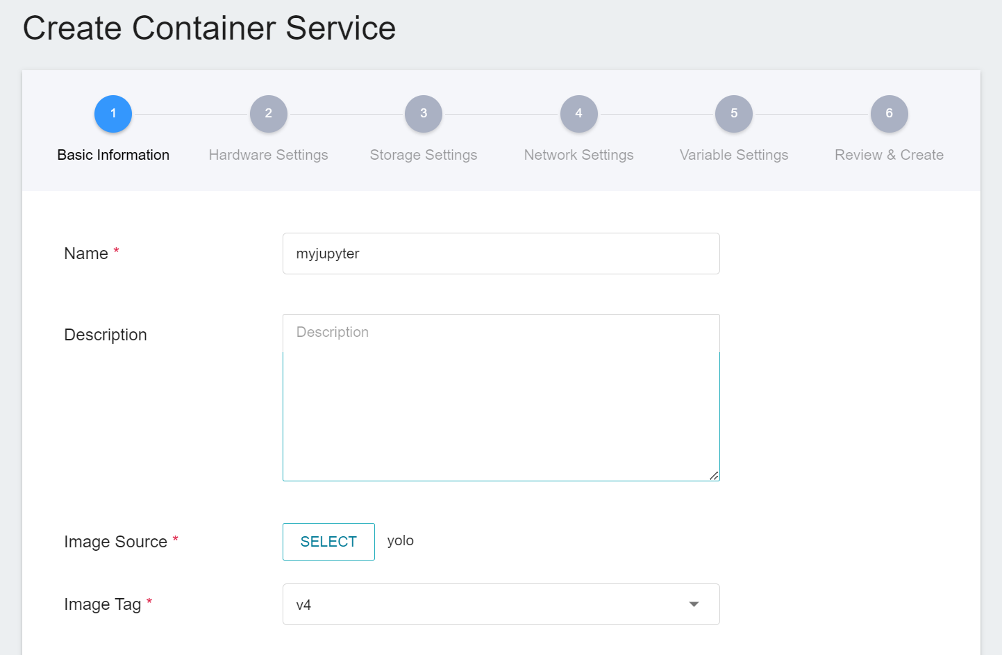
1. **Basic Information**
When creating a Container Service, you can directly select the **`yolo:v4`** image, in which we have provided the relevant environment of Jupyter Notebook.
2. **Hardware Settings**
Refer to the current available quota and program requirements, and select the appropriate hardware resources from the list. No need to configure the GPU here.
3. **Storage Settings**
This step can be skipped.
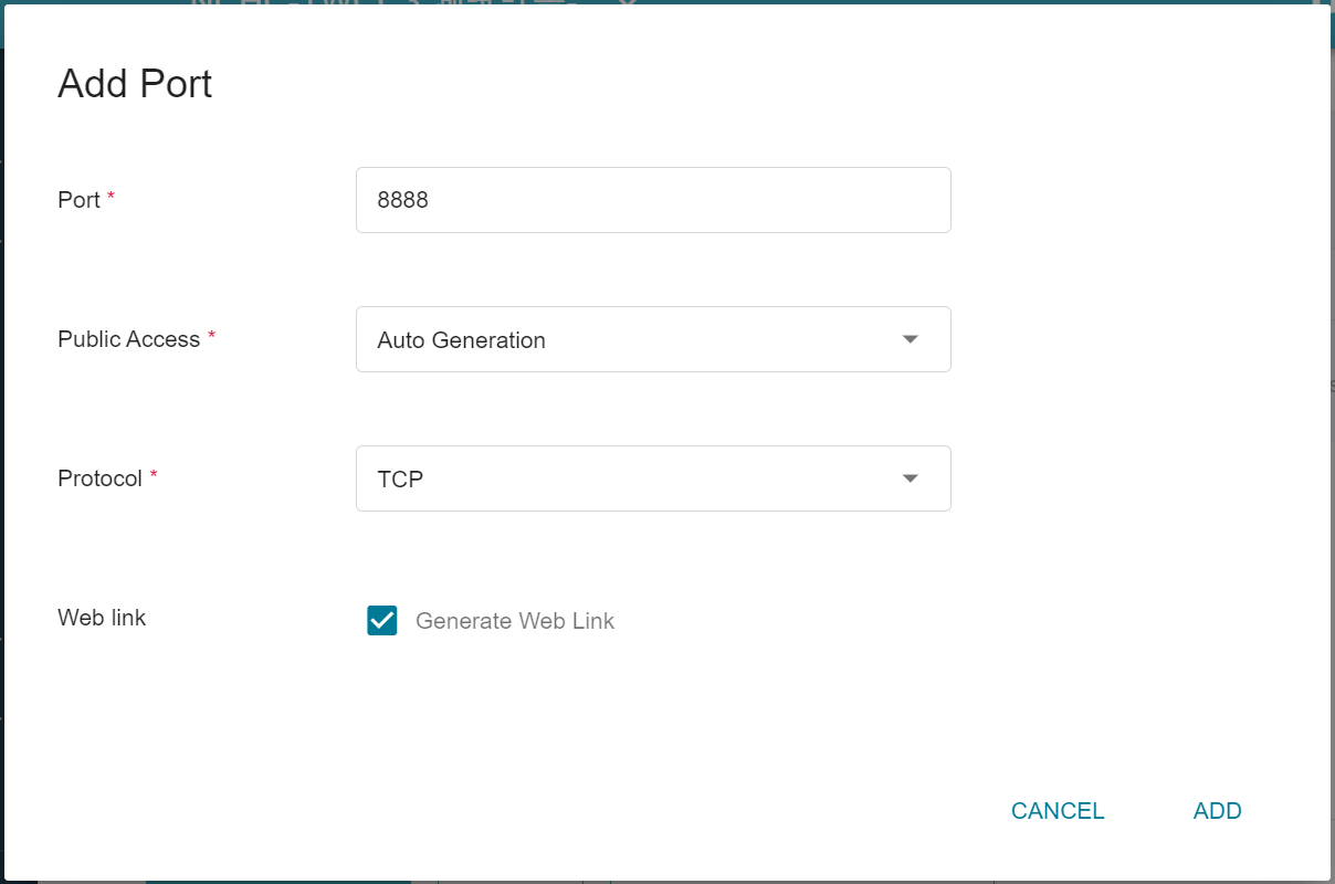
4. **Network Settings**
The Jupyter Notebook service runs on port 8888 by default. In order to access Jupyter Notebook from the outside, you need to set up an external public service port. You can chosse to let it automatically generate the Port for public access, by checking Generate Web Link.
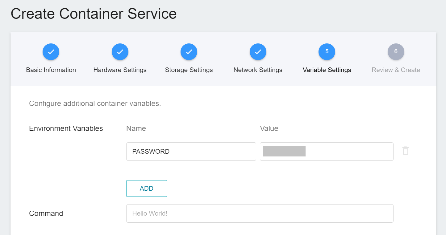
5. **Variable Settings**
To use Jupyter Notebook, you will need to enter a password. In this step, please use the environment variable **`PASSWORD`** preset in the image to set your own password.
6. **Review & Create**
Finally, confirm the entered information and click CREATE.
#### 5.1.2 **Use Jupyter Notebook**
After creating the Container Service, go back to the Container Service management list page and click on the service to get detailed information.
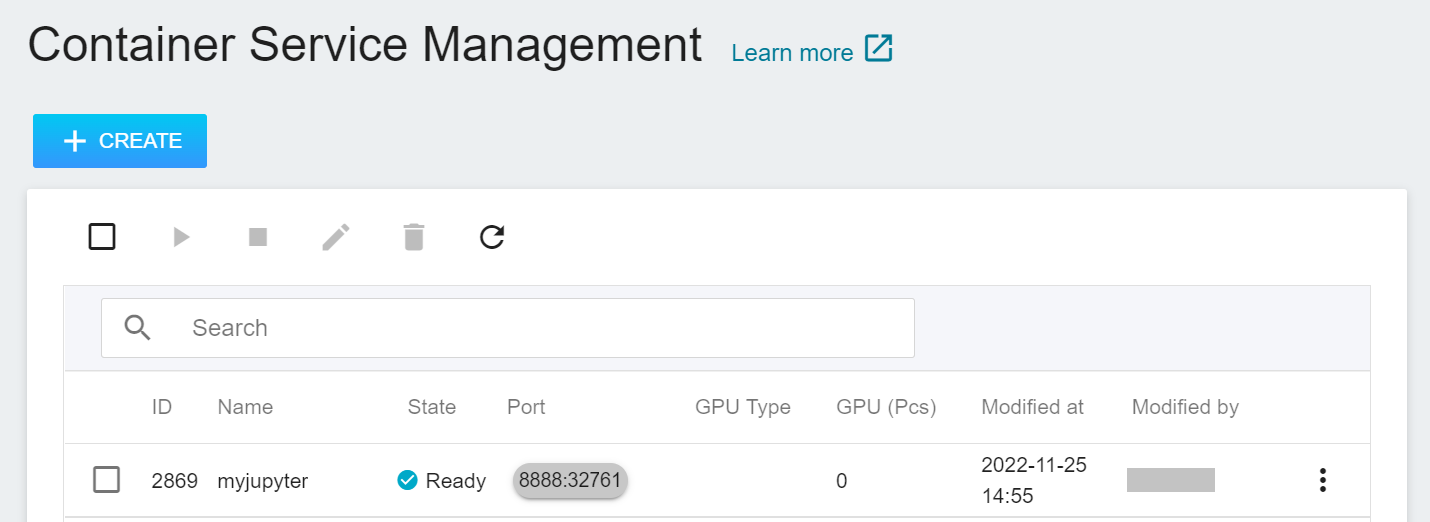
In the details page, you should pay special attention to the **Network** section, where there is an external service port `8888` for Jupyter Notebook, click the right side URL link to open Jupyter Notebook service in your browser.

When the login page of the Jupyter service appears, enter the **`PASSWORD`** variable value set in the **Variable Settings** step.
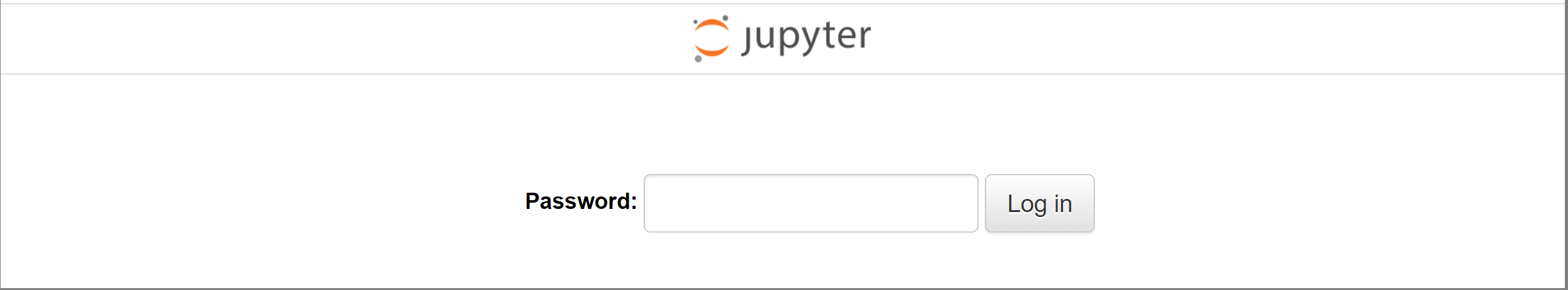
Now the Jupyter Notebook startup is complete.
### 5.2 Making Inferences
After opening Jupyter Notebook, you can see a program file called **`inference_client.ipynb`**, please modify this code according to your environment for inference. Below is a description of the code.
1. **Send Request**
This example uses the requests module to generate an HTTP POST request, and passes the image and parameters as a dictionary structure to the JSON parameter.
```python=1
# Default Dataset Path
datasetPath = "./test/"
# Inference Service Endpoint & Port
inferenceIP = "myinference-i"
inferencePort = "9999"
# Get All Files And Subdirectory Names
files = listdir(datasetPath)
for f in files:
fullpath = join(datasetPath, f)
if isfile(fullpath):
OUTPUT = join(resultPath, f)
with open(fullpath, "rb") as inputFile:
data = inputFile.read()
body = {"image": base64.b64encode(data).decode("utf-8"), "thresh": 0.5, "getImage": False}
res = requests.post("http://" + inferenceIP +":" + inferencePort + "/darknet/detect", json=body)
detected = res.json()
objects = detected.get('results')
```
There are several variables that require special attention.
* **`inferenceIP`** and **`inferencePort`** need to be filled with the Web Link of the inference service.
The example's **`inferenceIP`** is **myinference-i**, **`inferencePort`** is **9999**.
* **`thresh`** The predicted confidence value must be greater than this value in order to be classified into this category.<br><br>
2. **Retrieve Results**
After the object detection is completed, the results are sent back in JSON format:
- **`results`**: an object array, including one or more object detection results. If no object can be detected, an empty array is returned.
- **`results.bounding`**: the result of each detected object, which also includes:
- **`height`**: bounding box height.
- **`width`**: bounding box width.
- **`x`**: the x-coordinate of the center point of the bounding box.
- **`y`**: the y-coordinate of the center point of the bounding box.
- **`results.name`**: the classification result of this object.
- **`results.score`**: the confidence score for the classification of this object.
Once we have this information, we can draw the bounding accordingly.
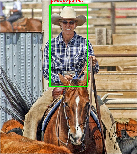
Based on these two programs, a request can be sent to the inference service, and the detection results can be retrieved and plotted on the original image.
### 5.3 Attached Code
:::spoiler **Program Code**
```python=1
import numpy as np
import base64
import io
import requests
import json
from PIL import Image as Images,ImageFont,ImageDraw
from IPython.display import Image, clear_output, display
import cv2
%matplotlib inline
from matplotlib import pyplot as plt
import time
from os import listdir
from os.path import isfile, isdir, join
datasetPath = "./test/"
resultPath = "./result/"
inferenceIP = "myinference-i"
inferencePort = "9999"
#Font setup
fontpath = "/notebooks/cht.otf"
color = (255, 0, 0)
font = ImageFont.truetype(fontpath, 20)
def arrayShow(imageArray):
resized = cv2.resize(imageArray, (500, 333), interpolation=cv2.INTER_CUBIC)
ret, png = cv2.imencode('.png', resized)
return Image(data=png)
# Get All Files And Subdirectory Names
files = listdir(datasetPath)
for f in files:
fullpath = join(datasetPath, f)
if isfile(fullpath):
OUTPUT = join(resultPath, f)
with open(fullpath, "rb") as inputFile:
data = inputFile.read()
body = {"image": base64.b64encode(data).decode("utf-8"), "thresh": 0.5, "getImage": False}
res = requests.post("http://" + inferenceIP +":" + inferencePort + "/darknet/detect", json=body)
detected = res.json()
objects = detected.get('results')
#print(detected)
for obj in objects:
bounding = obj.get('bounding')
name = obj.get('name')
height = bounding.get('height')
width = bounding.get('width')
score = obj.get('score')
detect_log = 'class:{!s} confidence:{!s}'.format(str(name), str(score))
#print(detect_log)
#Image(filename=FILE, width=600)
oriImage = cv2.imread(fullpath)
img_pil = Images.fromarray(cv2.cvtColor(oriImage, cv2.COLOR_BGR2RGB))
draw = ImageDraw.Draw(img_pil)
for obj in objects:
bounding = obj.get('bounding')
name = obj.get('name')
height = bounding.get('height')
width = bounding.get('width')
left = bounding.get('x') - (width/2)
top = bounding.get('y') - (height/2)
right = bounding.get('x') + (width/2)
bottom = bounding.get('y') + (height/2)
pos = (int(left), int(max((top - 10),0)))
box = (int(left), int(top)), (int(right), int(bottom))
draw.text(pos, name, font = font, fill = color)
draw.rectangle(box,outline="green")
cv_img = cv2.cvtColor(np.asarray(img_pil),cv2.COLOR_RGB2BGR)
cv2.imwrite(OUTPUT, cv_img)
img = arrayShow(cv_img)
clear_output(wait=True)
display(img)
#plt.imshow(oriImage)
#Image(filename=OUTPUT, width=600)
time.sleep(1)
```
:::
## 6. CVAT Assisted Annotation
CVAT has assisted annotation function to save time in manual annotation. As deep learning model is required to use CVAT to provide assisted annotation, you can train your own deep learning model by referring to the [**Training YOLO Model**](#3-Training-YOLO-Model). This section will introduce how to use the trained deep learning model to perform assisted annotation of image data with CVAT annotation tool.
### 6.1. Create YOLOv4 Assisted Annotation Service
The AI Maker system provides a **yolov4-cvat** inference template that allows you to quickly create assisted annotation inference services for the **yolov4 model**.
First, click **Inference** on the left to enter the **Inference Management** page, and click **+CREATE** to create an inference service.
1. **Basic Information**
Enter basic information about the inference service, select the **`yolov4-cvat`** template and choose the name and version of the model to be used for assisted annotation in the **Source Model**.
2. **Hardware Settings**
Select the appropriate hardware resource from the list with reference to the current available quota and training program requirements.
:::info
:bulb: **Tips:** For a better and faster experience with the assisted annotation function, please select the hardware option with GPU for the hardware settings.
:::
3. **Storage Settings**
No configuration is required for this step.
4. **Variable Settings**
In the Variable Settings page, these commands and parameters are automatically brought in when the **`yolov4-cvat`** template is applied.
5. **Subsequent Steps**
The subsequent steps are similar to those of other tasks and will not be repeated here.
### 6.2 Connect to CVAT
After you have created YOLOv4 assisted annotation inference service, you need to take another step to connect your inference service to CVAT. There are three places in AI Maker's inference service to connect to the CVAT service:
1. **CVAT Management** page
Click **Annotation Tools** on the left menu bar to enter the CVAT service home page. You need to click **ENABLE CVAT SERVICE** if you are using it for the first time. Only one CVAT service can be enabled for each project.
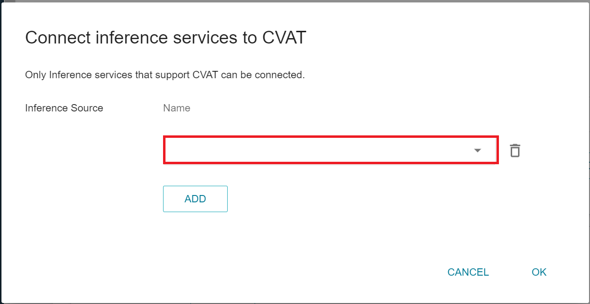
After entering the **CVAT Management** page, click the **ADD** button under the **Connect Inference Service to CVAT** section. If an existing inference service is connected to the CVAT, this button will change to **EDIT**.
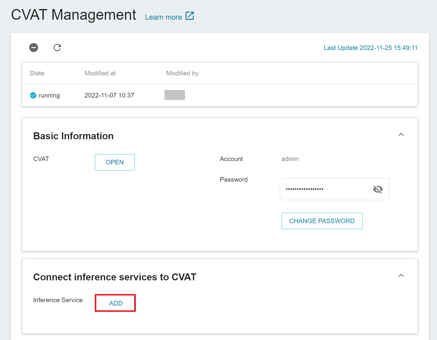
After the **Connect Inference Service to CVAT** window appears, select the inference service you want to connect to.
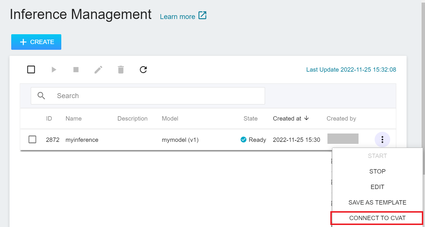
2. **Inference Management** page
Click **Inference** on the left function bar to enter **Inference Management**, move the mouse to the more options icon on the right side of automatic annotation task, and then click **CONNECT TO CVAT**.
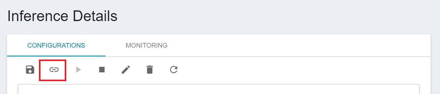
3. **Inference Details** page
Click the inference task list you want to connect to CVAT, enter the **Inference Details** page, and then click the **CONNECT TO CVAT** icon above.
### 6.3 Use CVAT Assisted Annotation Function
After you have completed the above steps, you can then log in to CVAT to use the assisted annotation function. Please refer to the instructions below for the steps:
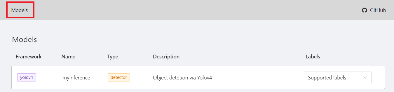
1. View CVAT Model
After entering the CVAT service page, click **MODELS** at the top, and you can see the inference service you just connected to CVAT.
2. Enable Assisted Annotation Function
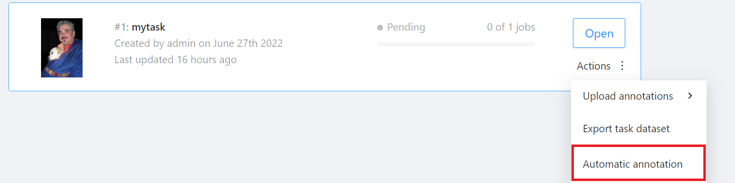
Go to the **Tasks** page and find the Task you want to annotate, then move the mouse over the More options icon in **Actions** to the right of the Task you want to annotate automatically, and then click **AUTOMATIC ANNOTATION**.
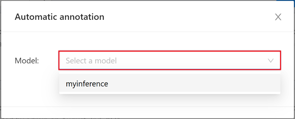
On the **Automatic Annotation** window that appears, click the **MODEL** drop-down menu and select the connected inference task.
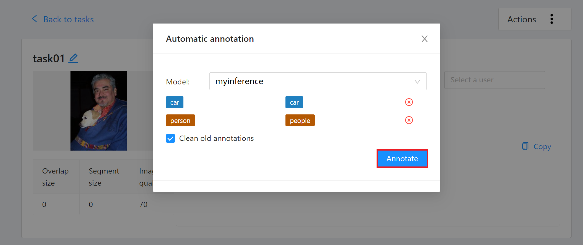
Then set the model to correspond to the task Label, and finally click **ANNOTATE** to perform automatic annotation.
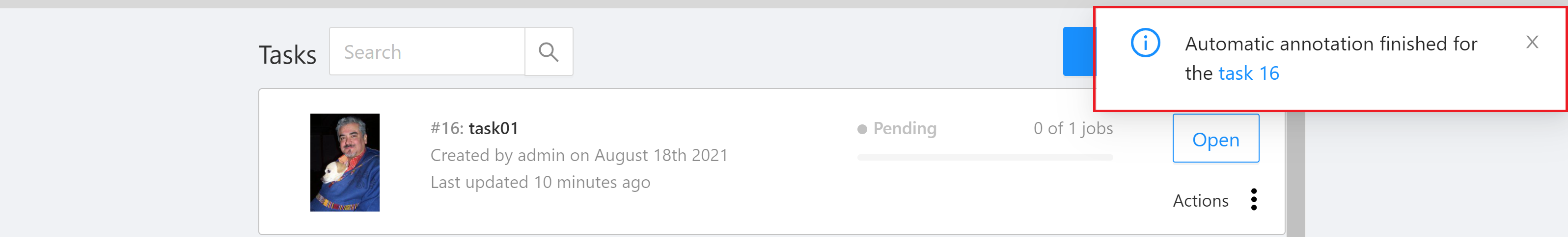
Once the automatic annotation task has started, you can see the percentage of completion. It will take some time to annotate a large amount of data, and a message will appear on the screen after the annotation is completed.
After the annotation is completed, enter the CVAT Annotation Tools page to view the automatic annotation result. If you are not satisfied with the result, you can perform manual annotation correction or retrain and optimize the model.